library(scTypeEval)
library(Matrix)scTypeEval: Evaluating Cell Type Labels Consistency in scRNA-seq
1 Introduction
Accurate cell type annotation is essential but challenging in single-cell RNA sequencing (scRNA-seq). Manual approaches are time-consuming, subjective, and inconsistent, while automated classifiers often fail to generalize across tissues, conditions, or closely related cell types. A key limitation for both is the lack of true ground truth for benchmarking.
scTypeEval provides a ground-truth-agnostic framework to systematically assess annotation quality using internal validation metrics. It enables:
- Quantification of inter-sample label consistency
- Identification of ambiguous or misclassified populations
- Reproducible benchmarking of manual annotations, automated classifiers, or clustering results
1.1 Key Features
- Ground-truth agnostic – Evaluate annotations without external references
- Cross-dataset benchmarking – Assess consistency across samples and studies
- Customizable – Works with Seurat, SingleCellExperiment, or matrices; supports custom gene lists
- Robust – Sensitive to misclassification; reliable across batch effects, label granularity, and sample sizes
2 Quick Start
Load the package:
2.1 Generate Example Data
For this vignette, we’ll create a synthetic dataset representing single-cell RNA-seq data from multiple samples with distinct cell types. This simulates a typical scenario where we want to evaluate the consistency of cell type annotations across biological replicates.
set.seed(22)

# Number of genes and cells
n_genes <- 5000
n_cells_per_sample <- 500
n_samples <- 6
cell_types <- c("CD4_T", "CD8_T", "B_cells", "NK_cells")

# Generate gene names
gene_names <- paste0("Gene_", seq_len(n_genes))

# Total cells
total_cells <- n_cells_per_sample * n_samples

# Generate metadata: samples and cell types
samples <- rep(paste0("Sample", seq_len(n_samples)), each = n_cells_per_sample)

# Assign cell types evenly within each sample
n_cell_types <- length(cell_types)
cells_per_type <- n_cells_per_sample %/% n_cell_types
celltypes <- rep(rep(cell_types, each = cells_per_type), times = n_samples)

# Initialize count matrix
count_matrix <- matrix(0, nrow = n_genes, ncol = total_cells)
rownames(count_matrix) <- gene_names
colnames(count_matrix) <- paste0("Cell_", seq_len(total_cells))

# Add cell-type-specific expression patterns
for (i in seq_along(cell_types)) {
  ct <- cell_types[i]
  ct_indices <- which(celltypes == ct)

  # Marker genes for this cell type (50 genes per type)
  marker_start <- ((i - 1) * 50 + 1)
  marker_end <- min(marker_start + 49, n_genes)
  marker_genes <- marker_start:marker_end

  # High expression in marker genes (lambda = 50)
  count_matrix[marker_genes, ct_indices] <- matrix(
    rpois(length(marker_genes) * length(ct_indices), lambda = 50),
    nrow = length(marker_genes)
  )

  # Background expression in other genes (lambda = 5)
  other_genes <- setdiff(seq_len(n_genes), marker_genes)
  count_matrix[other_genes, ct_indices] <- matrix(
    rpois(length(other_genes) * length(ct_indices), lambda = 5),
    nrow = length(other_genes)
  )
}

# Add sample-specific batch effects
for (s in seq_len(n_samples)) {
  sample_cells <- which(samples == paste0("Sample", s))
  batch_effect <- rnorm(1, mean = 1, sd = 0.1)
  count_matrix[, sample_cells] <- round(
    count_matrix[, sample_cells] * batch_effect
  )
}

# Convert to sparse matrix
count_matrix <- Matrix(count_matrix, sparse = TRUE)

# Create metadata dataframe
metadata <- data.frame(
  celltype = celltypes,
  sample = samples,
  batch = rep(
    c("Batch1", "Batch2"),
    each = n_cells_per_sample * (n_samples/2)
  ),
  row.names = colnames(count_matrix),
  stringsAsFactors = FALSE
)

# Preview the data
head(metadata)
#>        celltype  sample  batch
#> Cell_1    CD4_T Sample1 Batch1
#> Cell_2    CD4_T Sample1 Batch1
#> Cell_3    CD4_T Sample1 Batch1
#> Cell_4    CD4_T Sample1 Batch1
#> Cell_5    CD4_T Sample1 Batch1
#> Cell_6    CD4_T Sample1 Batch1
dim(count_matrix)
#> [1] 5000 3000
3 Core Workflow
3.1 Step 1: Create scTypeEval Object
scTypeEval objects can be created from:
- A count matrix and metadata dataframe
- A Seurat object
- A SingleCellExperiment object
# Create scTypeEval object from matrix and metadata
sceval <- create_scTypeEval(
  matrix = count_matrix,
  metadata = metadata
)
The scTypeEval object stores the raw count data and metadata, which will be processed in subsequent steps.
3.2 Step 2: Process Data
Process and normalize the data, creating both single-cell and pseudobulk representations. This step:
- Aggregates counts by cell type and sample (pseudobulk)
- Filters out cell types with insufficient samples or cells
- Normalizes the data for downstream analysis
# Process data with filtering criteria
sceval <- run_processing_data(
  scTypeEval = sceval,
  ident = "celltype",          # Column defining cell type identities
  sample = "sample",           # Column defining sample IDs
  min_samples = 3,             # Minimum samples required per cell type
  min_cells = 10               # Minimum cells per sample-celltype combination
)
The processed data is stored as data_assay objects within the scTypeEval object, accessible for downstream analysis.
3.3 Step 3: Extract Relevant Features
Identify biologically relevant features for evaluating consistency. scTypeEval supports:
- Highly Variable Genes (HVGs): Genes with high variability across the dataset
- Cell Type Marker Genes: Genes differentially expressed in each cell type
- Custom Gene Lists: User-defined gene sets
3.3.1 Highly Variable Genes
# Identify HVGs using the basic method
sceval <- run_hvg(
  scTypeEval = sceval,
  var_method = "basic", # Method for variance modeling: "basic" or "scran"
  ngenes = 1000,        # Number of HVGs to retain
  sample = TRUE         # Perform sample-level blocking
)

# View stored gene lists
gene_lists <- sceval@gene_lists
names(gene_lists)
#> [1] "HVG"
if ("HVG" %in% names(gene_lists)) {
  length(gene_lists$HVG)
}
#> [1] 1000
3.3.2 Cell Type Marker Genes
# Identify marker genes per cell type
sceval <- run_gene_markers(
  scTypeEval = sceval,
  method = "scran.findMarkers",  # Method for finding markers
  ngenes_celltype = 50           # Maximum markers per cell type
)

# View marker genes
gene_lists <- sceval@gene_lists
if (!is.null(gene_lists$scran.findMarkers)) {
  head(gene_lists$scran.findMarkers, 20)
}
#>  [1] "Gene_119" "Gene_131" "Gene_125" "Gene_104" "Gene_149" "Gene_129"
#>  [7] "Gene_147" "Gene_138" "Gene_133" "Gene_103" "Gene_112" "Gene_128"
#> [13] "Gene_121" "Gene_115" "Gene_148" "Gene_107" "Gene_116" "Gene_124"
#> [19] "Gene_110" "Gene_143"
3.3.3 Custom Gene Lists (Optional)
You can also add custom gene lists using add_gene_list():
# Example: Add a custom list of immune response genes
custom_genes <- c("Gene_1", "Gene_50", "Gene_100", "Gene_150")

sceval <- add_gene_list(
  scTypeEval = sceval,
  gene_list = list("custom_genes" = custom_genes)
)
These different selected features are stored within the scTypeEval object and can be used in the subsequent steps.
gene_lists <- sceval@gene_lists
names(gene_lists)
#> [1] "HVG"               "scran.findMarkers" "custom_genes"
3.4 Step 4: Dimensional Reduction (Optional but Recommended)
Consistency metrics can be computed directly on the selected features. However, computing them in a low-dimensional space (e.g., PCA) significantly speeds up the analysis while yielding similar results.
# Run PCA on processed data
sceval <- run_pca(
  scTypeEval = sceval,
  ndim = 20,         # Number of principal components
  gene_list = "HVG" # specify gene list to subset if multiple were added
)

# View available reductions
reductions <- sceval@reductions
if (length(reductions) > 0) {
  names(reductions)
}
#> [1] "single-cell" "pseudobulk"
Alternatively, pre-computed embeddings (PCA, UMAP, t-SNE) can be inserted using add_dim_reduction().
3.5 Step 5: Compute Dissimilarity Matrices
The core of scTypeEval is computing pairwise dissimilarities between cell types across samples. Multiple dissimilarity methods are supported:
3.5.1 Pseudobulk-based Distances
Compute distances between pseudobulk gene expression profiles:
# Euclidean distance on pseudobulk profiles
sceval <- run_dissimilarity(
  sceval,
  method = "Pseudobulk:Euclidean",
  reduction = FALSE # Use processed expression data of selected features
)

# Cosine distance on PCA embeddings
sceval <- run_dissimilarity(
  sceval,
  method = "Pseudobulk:Cosine",
  reduction = TRUE               # Use PCA space
)
3.5.2 Wasserstein Distance
Compute Wasserstein distances between single-cell distributions:
# Wasserstein distance on PCA embeddings (faster)
sceval <- run_dissimilarity(
  sceval,
  method = "WasserStein",
  reduction = TRUE
)
3.5.3 Reciprocal Classification
Match cells across samples using a classifier:
# Reciprocal classification with SingleR
sceval <- run_dissimilarity(
  sceval,
  method = "recip_classif:Match",
  reciprocal_classifier = "SingleR",
  # usage of dimensional reduction not supported
  # for this dissimilarity approach
  reduction = FALSE
)
3.5.4 View Available Dissimilarity Matrices
# List all computed dissimilarity matrices
dissim <- sceval@dissimilarity
if (length(dissim) > 0) {
  names(dissim)
}
#> [1] "Pseudobulk:Euclidean" "Pseudobulk:Cosine"    "WasserStein"
#> [4] "recip_classif:Match"
3.6 Step 6: Compute Consistency Metrics
Evaluate inter-sample consistency for each cell type using internal validation metrics. scTypeEval supports multiple consistency metrics:
- silhouette: Standard cohesion/separation score
- 2label_silhouette: Silhouette comparing “own type” vs. all others
- NeighborhoodPurity: Fraction of K-nearest neighbors with same label
- ward_PropMatch: Proportion in dominant Ward cluster
- Orbital_medoid: Fraction closer to own medoid than others
- Average_similarity: Within-type similarity vs. between-type
3.6.1 Compute Silhouette Scores
# Compute silhouette consistency on Euclidean dissimilarity
consistency_sil <- get_consistency(
  sceval,
  dissimilarity_slot = "Pseudobulk:Euclidean",
  consistency_metric = "silhouette"
)

# View results
print(consistency_sil)
#>          celltype   measure consistency_metric dissimilarity_method    ident
#> CD4.T       CD4.T 0.9392103         silhouette Pseudobulk:Euclidean celltype
#> CD8.T       CD8.T 0.9372690         silhouette Pseudobulk:Euclidean celltype
#> B.cells   B.cells 0.9382785         silhouette Pseudobulk:Euclidean celltype
#> NK.cells NK.cells 0.9370830         silhouette Pseudobulk:Euclidean celltype
Higher values indicate better consistency (samples with the same cell type annotation are more similar to each other than to samples with different annotations).
3.6.2 Compute Neighborhood Purity
# Compute neighborhood purity on Wasserstein dissimilarity
consistency_nbhd <- get_consistency(
  sceval,
  dissimilarity_slot = "WasserStein",
  consistency_metric = "NeighborhoodPurity"
)

# View results
print(consistency_nbhd)
#>          celltype measure consistency_metric dissimilarity_method    ident
#> CD4.T       CD4.T       1 NeighborhoodPurity          WasserStein celltype
#> CD8.T       CD8.T       1 NeighborhoodPurity          WasserStein celltype
#> B.cells   B.cells       1 NeighborhoodPurity          WasserStein celltype
#> NK.cells NK.cells       1 NeighborhoodPurity          WasserStein celltype
3.6.3 Compare Multiple Metrics
consistency_all <-
  get_consistency(
    sceval,
    dissimilarity_slot = c("Pseudobulk:Euclidean",
                           "WasserStein"), # allow multiple arguments
    consistency_metric = c("silhouette",
                           "NeighborhoodPurity",
                           "Average_similarity") # allow multiple arguments
  )

print(consistency_all)
#>            celltype   measure consistency_metric dissimilarity_method    ident
#> CD4.T         CD4.T 0.9392103         silhouette Pseudobulk:Euclidean celltype
#> CD8.T         CD8.T 0.9372690         silhouette Pseudobulk:Euclidean celltype
#> B.cells     B.cells 0.9382785         silhouette Pseudobulk:Euclidean celltype
#> NK.cells   NK.cells 0.9370830         silhouette Pseudobulk:Euclidean celltype
#> CD4.T1        CD4.T 1.0000000 NeighborhoodPurity Pseudobulk:Euclidean celltype
#> CD8.T1        CD8.T 1.0000000 NeighborhoodPurity Pseudobulk:Euclidean celltype
#> B.cells1    B.cells 1.0000000 NeighborhoodPurity Pseudobulk:Euclidean celltype
#> NK.cells1  NK.cells 1.0000000 NeighborhoodPurity Pseudobulk:Euclidean celltype
#> CD4.T2        CD4.T 0.9427627 Average_similarity Pseudobulk:Euclidean celltype
#> CD8.T2        CD8.T 0.9410225 Average_similarity Pseudobulk:Euclidean celltype
#> B.cells2    B.cells 0.9419125 Average_similarity Pseudobulk:Euclidean celltype
#> NK.cells2  NK.cells 0.9408865 Average_similarity Pseudobulk:Euclidean celltype
#> CD4.T3        CD4.T 0.9008518         silhouette          WasserStein celltype
#> CD8.T3        CD8.T 0.9009151         silhouette          WasserStein celltype
#> B.cells3    B.cells 0.8998458         silhouette          WasserStein celltype
#> NK.cells3  NK.cells 0.8996690         silhouette          WasserStein celltype
#> CD4.T11       CD4.T 1.0000000 NeighborhoodPurity          WasserStein celltype
#> CD8.T11       CD8.T 1.0000000 NeighborhoodPurity          WasserStein celltype
#> B.cells11   B.cells 1.0000000 NeighborhoodPurity          WasserStein celltype
#> NK.cells11 NK.cells 1.0000000 NeighborhoodPurity          WasserStein celltype
#> CD4.T21       CD4.T 0.9099102 Average_similarity          WasserStein celltype
#> CD8.T21       CD8.T 0.9099267 Average_similarity          WasserStein celltype
#> B.cells21   B.cells 0.9090413 Average_similarity          WasserStein celltype
#> NK.cells21 NK.cells 0.9089435 Average_similarity          WasserStein celltype
4 Visualization
4.1 Dissimilarity Heatmap
Visualize dissimilarity matrices as annotated heatmaps. Cell types can be ordered by similarity or consistency scores:
# Plot dissimilarity heatmap with consistency-based ordering
plot_heatmap(
  sceval,
  dissimilarity_slot = "Pseudobulk:Euclidean",
  sort_consistency = "silhouette",      # Order by silhouette scores
  sort_similarity = NULL                 # Or order by similarity
)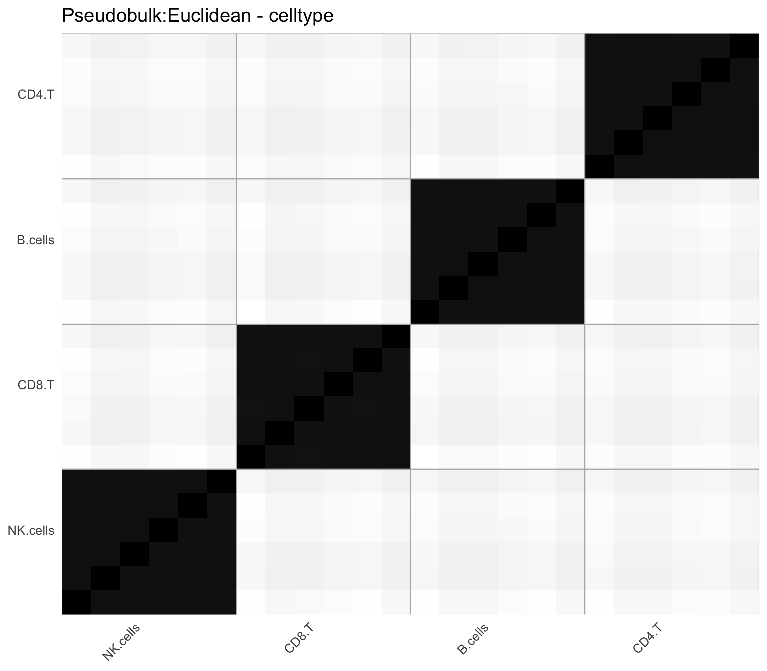
The heatmap shows pairwise dissimilarities between samples, grouped by cell type. Cell types with higher consistency (e.g., more coherent annotations) show tighter clustering of their samples.
4.2 Pseudobulk PCA
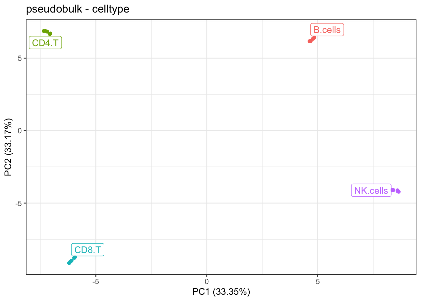
Pseudobulk PCA per sample & cell type
plot_pca(
  sceval,
  reduction_slot = "pseudobulk"
)
5 Interpretation Guidelines
5.1 Identifying Problematic Annotations
Cell types with low consistency scores may indicate:
- Ambiguous cell type boundaries: Related cell types (e.g., activated vs. resting T cells) may overlap
- Heterogeneous populations: A single label covering multiple biological states
- Annotation errors: Inconsistent labeling across samples
5.2 Recommendations
- Investigate cell types with low consistency using the heatmap visualization
- Consider refining annotations for cell types with negative consistency scores
- Use biological knowledge to interpret whether low consistency reflects true biology or annotation issues
6 Session Information
sessionInfo()
#> R version 4.6.0 alpha (2026-03-31 r89754)
#> Platform: aarch64-apple-darwin23
#> Running under: macOS Tahoe 26.5.1
#>
#> Matrix products: default
#> BLAS:   /Library/Frameworks/R.framework/Versions/4.6/Resources/lib/libRblas.0.dylib
#> LAPACK: /Library/Frameworks/R.framework/Versions/4.6/Resources/lib/libRlapack.dylib;  LAPACK version 3.12.1
#>
#> locale:
#> [1] en_US.UTF-8/en_US.UTF-8/en_US.UTF-8/C/en_US.UTF-8/en_US.UTF-8
#>
#> time zone: Europe/Zurich
#> tzcode source: internal
#>
#> attached base packages:
#> [1] stats     graphics  grDevices datasets  utils     methods   base
#>
#> other attached packages:
#> [1] Matrix_1.7-5     scTypeEval_1.0.0
#>
#> loaded via a namespace (and not attached):
#>  [1] SummarizedExperiment_1.42.0 transport_0.15-4
#>  [3] gtable_0.3.6                ggplot2_4.0.3
#>  [5] xfun_0.60                   htmlwidgets_1.6.4
#>  [7] ggrepel_0.9.8               Biobase_2.72.0
#>  [9] lattice_0.22-9              vctrs_0.7.3
#> [11] tools_4.6.0                 generics_0.1.4
#> [13] stats4_4.6.0                parallel_4.6.0
#> [15] tibble_3.3.1                SingleR_2.14.0
#> [17] cluster_2.1.8.2             pkgconfig_2.0.3
#> [19] BiocNeighbors_2.6.0         data.table_1.18.4
#> [21] RColorBrewer_1.1-3          S7_0.2.2
#> [23] S4Vectors_0.50.1            dqrng_0.4.1
#> [25] lifecycle_1.0.5             farver_2.1.2
#> [27] compiler_4.6.0              statmod_1.5.2
#> [29] bluster_1.22.0              Seqinfo_1.2.0
#> [31] codetools_0.2-20            htmltools_0.5.9
#> [33] yaml_2.3.12                 pillar_1.11.1
#> [35] BiocParallel_1.46.0         SingleCellExperiment_1.34.0
#> [37] DelayedArray_0.38.2         limma_3.68.4
#> [39] abind_1.4-8                 tidyselect_1.2.1
#> [41] rsvd_1.0.5                  locfit_1.5-9.12
#> [43] metapod_1.20.0              digest_0.6.39
#> [45] BiocSingular_1.28.0         dplyr_1.2.1
#> [47] labeling_0.4.3              fastmap_1.2.0
#> [49] grid_4.6.0                  cli_3.6.6
#> [51] SparseArray_1.12.2          magrittr_2.0.5
#> [53] S4Arrays_1.12.0             withr_3.0.3
#> [55] edgeR_4.10.1                scales_1.4.0
#> [57] rmarkdown_2.31              XVector_0.52.0
#> [59] matrixStats_1.5.0           igraph_2.3.3
#> [61] otel_0.2.0                  scran_1.40.0
#> [63] ScaledMatrix_1.20.0         beachmat_2.28.0
#> [65] evaluate_1.0.5              knitr_1.51
#> [67] GenomicRanges_1.64.0        IRanges_2.46.0
#> [69] irlba_2.3.7                 rlang_1.3.0
#> [71] Rcpp_1.1.2                  glue_1.8.1
#> [73] scuttle_1.22.0              renv_1.2.3
#> [75] BiocGenerics_0.58.1         jsonlite_2.0.0
#> [77] R6_2.6.1                    MatrixGenerics_1.24.0
7 References
The manuscript describing these methods is currently in preparation. For questions or issues, please visit:
- GitHub: https://github.com/carmonalab/scTypeEval
- Bug reports: https://github.com/carmonalab/scTypeEval/issues