library(scTypeEval)
library(Matrix)
library(dplyr)
library(tidyr)
library(ggplot2)Diagnostics of low consistent annotations
1 Goal
This tutorial uses a real PBMC dataset to show, step by step, how to compute and interpret the two recommended ISC diagnostics:
- Local ISC (ISCL) =
silhouetteonrecip_classif:Match - Global ISC (ISCG) =
2label_silhouetteonPseudobulk:Cosine
We then introduce two controlled annotation perturbations:
- split one label (
B_cell) to induce local inconsistency - merge two labels (
CD14+B_cell) to induce global inconsistency
2 Dataset description
The input object is: PBMC_Cambridge_Healthy_33879890
It was generated by: make_PBMC_Stephenson.R
Based on that script, the dataset was obtained as follows:
- download the full Stephenson PBMC object from Zenodo (
Stephenson_2021_33879890.rds) - keep only Cambridge site and Healthy status
- keep only these author labels from
OriginalAnnotationLevel1:B_cell,CD4,NK_16hi,CD14,DCs
- retain only the columns needed for ISC:
- sample of origin:
Sample - annotation:
OriginalAnnotationLevel1
- sample of origin:
- remove blacklisted genes (TCR, immunoglobulins, Y genes)
- keep top variable genes (4000) and save a light object with:
countsmetadata
3 Load packages
4 Load the real PBMC dataset
url <- "https://raw.githubusercontent.com/carmonalab/scTypeEval_CaseStudies/master/datasets/PBMC_Cambridge_Healthy_33879890.rds"
cache_dir <- file.path("../datasets")
dir.create(cache_dir, recursive = TRUE, showWarnings = FALSE)
dataset_file <- file.path(
  cache_dir,
  "PBMC_Cambridge_Healthy_33879890.rds"
)
if (!file.exists(dataset_file)) {
  utils::download.file(url, dataset_file, mode = "wb")
}
infile <- "../datasets/PBMC_Cambridge_Healthy_33879890.rds"
pbmc <- readRDS(infile)

counts <- pbmc$counts
metadata <- pbmc$metadata
5 Baseline annotation: explicit scTypeEval workflow
data(black_list)
blacklist_genes <- c(
  black_list$TCR,
  black_list$Immunoglobulins,
  black_list$Ygenes
)
5.1 Step 1: create scTypeEval object
sceval_baseline <- create_scTypeEval(
  matrix = counts,
  metadata = metadata
)
5.2 Step 2: process data
sceval_baseline <- run_processing_data(
  scTypeEval = sceval_baseline,
  ident = "OriginalAnnotationLevel1",
  sample = "Sample",
  min_samples = 5,
  min_cells = 10
)
5.3 Step 3: select HVGs
sceval_baseline <- run_hvg(
  scTypeEval = sceval_baseline,
  var_method = "scran",
  ngenes = 1200,
  sample = TRUE,
  aggregation = "single-cell",
  black_list = blacklist_genes
)
5.4 Step 4: run PCA
sceval_baseline <- run_pca(
  scTypeEval = sceval_baseline,
  ndim = 25
)

plot_pca(sceval_baseline)
#> $`single-cell`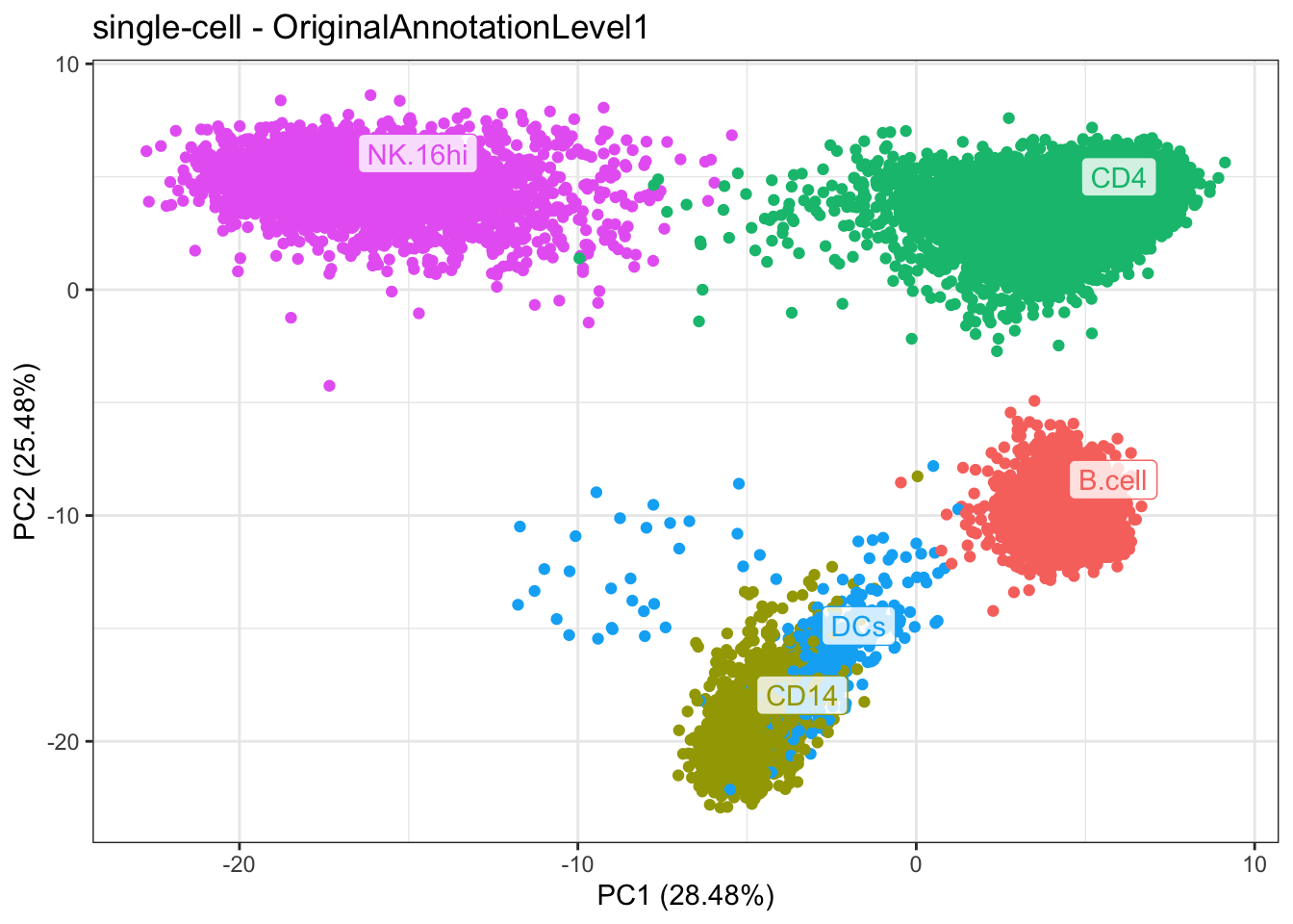
#>
#> $pseudobulk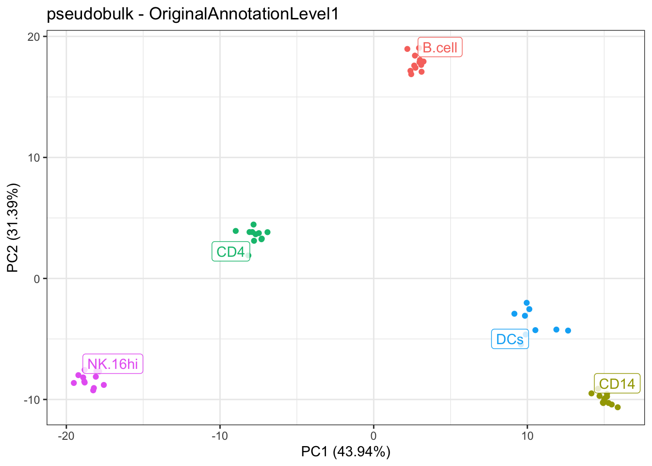
5.5 Step 5: compute dissimilarity matrices
sceval_baseline <- run_dissimilarity(
  sceval_baseline,
  method = "recip_classif:Match",
  reduction = FALSE
)

sceval_baseline <- run_dissimilarity(
  sceval_baseline,
  method = "Pseudobulk:Cosine",
  reduction = TRUE
)
5.6 Step 6: compute local and global ISC
isc_baseline_raw <- get_consistency(
  sceval_baseline,
  dissimilarity_slot = c("recip_classif:Match", "Pseudobulk:Cosine"),
  consistency_metric = c("silhouette", "2label_silhouette")
)

scores_baseline <- isc_baseline_raw |>
  mutate(method.type = paste(consistency_metric, dissimilarity_method, sep = " | ")) |>
  filter(method.type %in% c(
    "silhouette | recip_classif:Match",
    "2label_silhouette | Pseudobulk:Cosine"
  )) |>
  mutate(
    metric = factor(
      method.type,
      levels = c(
        "silhouette | recip_classif:Match",
        "2label_silhouette | Pseudobulk:Cosine"
      ),
      labels = c("local_isc", "global_isc")
    )
  ) |>
  select(celltype, metric, measure) |>
  pivot_wider(names_from = metric, values_from = measure)

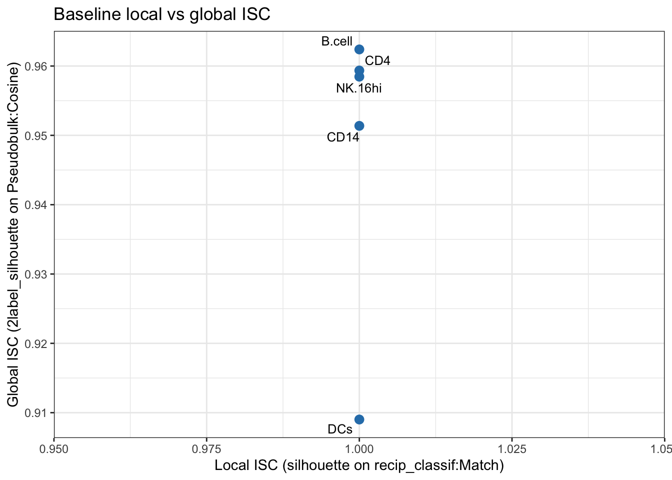
scores_baseline
#> # A tibble: 5 × 3
#>   celltype local_isc global_isc
#>   <chr>        <dbl>      <dbl>
#> 1 B.cell           1      0.962
#> 2 CD4              1      0.959
#> 3 NK.16hi          1      0.958
#> 4 CD14             1      0.951
#> 5 DCs 1 0.909ggplot(scores_baseline, aes(x = local_isc, y = global_isc, label = celltype)) +
geom_point(size = 2.8, color = "#2c7fb8") +
ggrepel::geom_text_repel(size = 3.4, max.overlaps = Inf) +
theme_bw() +
labs(
title = "Baseline local vs global ISC",
x = "Local ISC (silhouette on recip_classif:Match)",
y = "Global ISC (2label_silhouette on Pseudobulk:Cosine)"
) 
6 Scenario 1: split one label to decrease local ISC
We split B_cell into B_cell_A and B_cell_B without changing expression values.
metadata_split <- metadata |>
  group_by(Sample, OriginalAnnotationLevel1) |>
  mutate(rank_in_group = row_number()) |>
  ungroup() |>
  mutate(
    label_split = case_when(
      OriginalAnnotationLevel1 == "B_cell" & rank_in_group %% 2 == 0 ~ "B_cell_A",
      OriginalAnnotationLevel1 == "B_cell" & rank_in_group %% 2 == 1 ~ "B_cell_B",
      TRUE ~ OriginalAnnotationLevel1
    )
  ) |>
  select(-rank_in_group)

table(metadata_split$label_split)
#>
#> B_cell_A B_cell_B     CD14      CD4      DCs  NK_16hi
#>     1211     1216     1622    12207      393     3616
6.1 Re-run the same scTypeEval steps with split labels
sceval_split <- create_scTypeEval(
  matrix = counts,
  metadata = metadata_split
)

sceval_split <- run_processing_data(
  scTypeEval = sceval_split,
  ident = "label_split",
  sample = "Sample",
  min_samples = 3,
  min_cells = 20
)

sceval_split <- run_hvg(
  scTypeEval = sceval_split,
  var_method = "scran",
  ngenes = 1200,
  sample = TRUE,
  aggregation = "single-cell",
  black_list = blacklist_genes
)

sceval_split <- run_pca(
  scTypeEval = sceval_split,
  ndim = 25
)

sceval_split <- run_dissimilarity(
  sceval_split,
  method = "recip_classif:Match",
  reduction = FALSE
)

sceval_split <- run_dissimilarity(
  sceval_split,
  method = "Pseudobulk:Cosine",
  reduction = TRUE
)
isc_split_raw <- get_consistency(
sceval_split,
dissimilarity_slot = c("recip_classif:Match", "Pseudobulk:Cosine"),
consistency_metric = c("silhouette", "2label_silhouette")
)
scores_split <- isc_split_raw |>
mutate(method.type = paste(consistency_metric, dissimilarity_method, sep = " | ")) |>
filter(method.type %in% c(
"silhouette | recip_classif:Match",
"2label_silhouette | Pseudobulk:Cosine"
)) |>
mutate(
metric = factor(
method.type,
levels = c(
"silhouette | recip_classif:Match",
"2label_silhouette | Pseudobulk:Cosine"
),
labels = c("local_isc", "global_isc")
)
) |>
select(celltype, metric, measure) |>
pivot_wider(names_from = metric, values_from = measure)
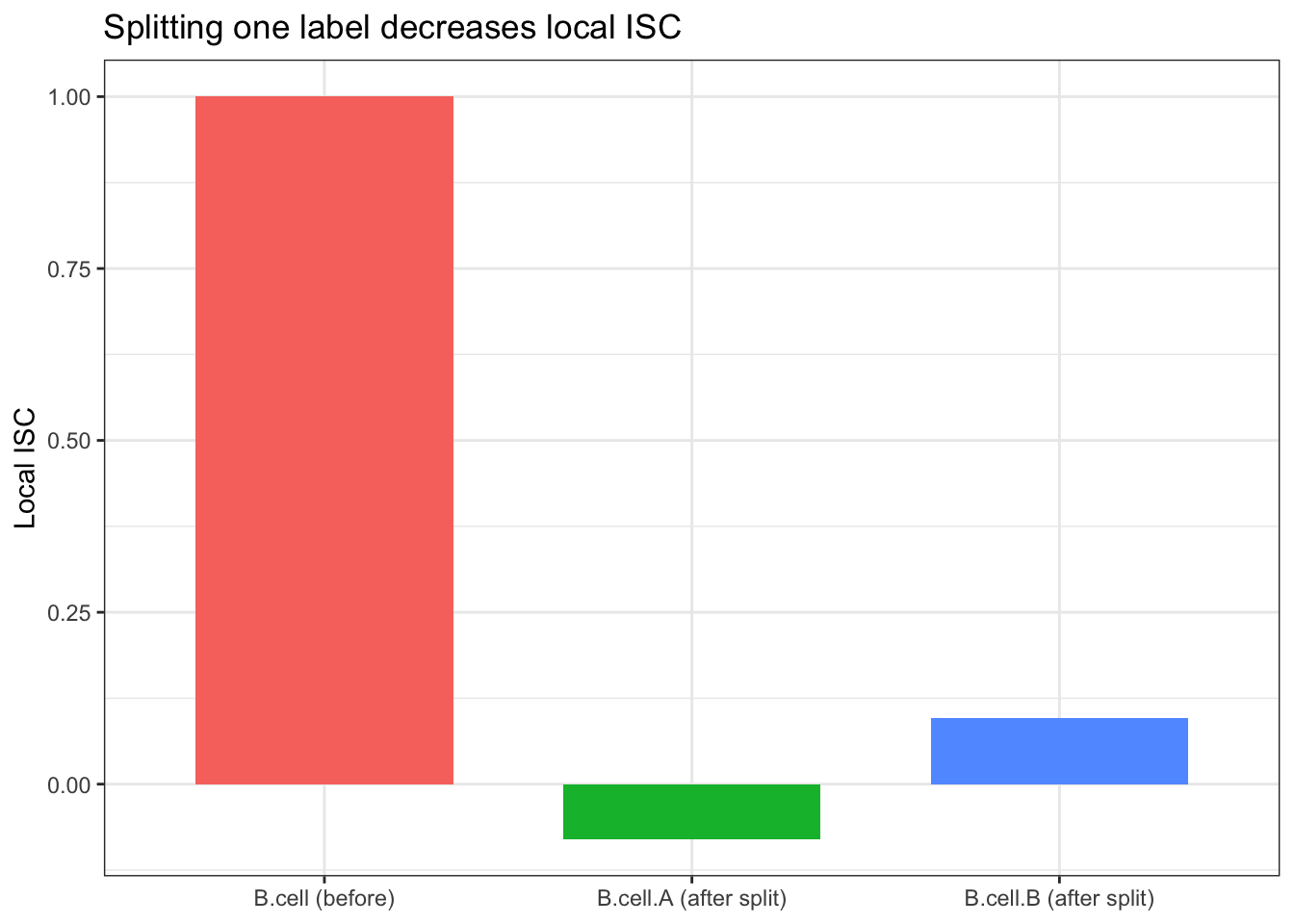
scores_split
#> # A tibble: 6 × 3
#> celltype local_isc global_isc
#> <chr> <dbl> <dbl>
#> 1 B.cell.B 0.0965 0.921
#> 2 CD4 1 0.967
#> 3 NK.16hi 1 0.967
#> 4 B.cell.A -0.0801 0.920
#> 5 CD14 1 0.961
#> 6 DCs 1 0.927before_local <- scores_baseline |>
filter(celltype == "B.cell") |>
transmute(target = "B.cell (before)", local_isc)
after_local <- scores_split |>
filter(celltype %in% c("B.cell.A", "B.cell.B")) |>
mutate(target = paste0(celltype, " (after split)")) |>
select(target, local_isc)
bind_rows(before_local, after_local) |>
ggplot(aes(x = target, y = local_isc, fill = target)) +
geom_col(width = 0.7, show.legend = FALSE) +
theme_bw() +
labs(
title = "Splitting one label decreases local ISC",
x = NULL,
y = "Local ISC"
)
7 Scenario 2: merge CD14 + B_cell to decrease global ISC
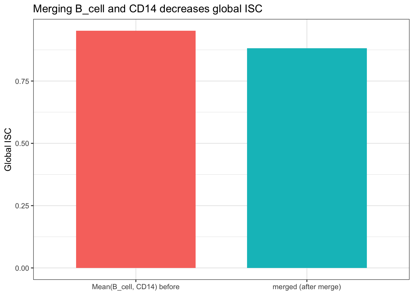
CD14 and B_cell represent distinct immune lineages (myeloid and lymphoid, respectively). Merging these biologically distinct populations creates a broader, more heterogeneous label, which is expected to decrease global compactness and separation, resulting in a lower global ISC score.
metadata_merge <- metadata |>
  mutate(
    label_merge = ifelse(OriginalAnnotationLevel1 %in% c("CD14", "B_cell"),
                         "merged",
                         as.character(OriginalAnnotationLevel1))
  )

table(metadata_merge$label_merge)
#>
#>     CD4     DCs  merged NK_16hi
#>   12207     393    4049    3616
7.1 Re-run the same scTypeEval steps with merged labels
sceval_merge <- create_scTypeEval(
  matrix = counts,
  metadata = metadata_merge
)

sceval_merge <- run_processing_data(
  scTypeEval = sceval_merge,
  ident = "label_merge",
  sample = "Sample",
  min_samples = 3,
  min_cells = 20
)

sceval_merge <- run_hvg(
  scTypeEval = sceval_merge,
  var_method = "scran",
  ngenes = 1200,
  sample = TRUE,
  aggregation = "single-cell",
  black_list = blacklist_genes
)

sceval_merge <- run_pca(
  scTypeEval = sceval_merge,
  ndim = 25
)

sceval_merge <- run_dissimilarity(
  sceval_merge,
  method = "recip_classif:Match",
  reduction = FALSE
)

sceval_merge <- run_dissimilarity(
  sceval_merge,
  method = "Pseudobulk:Cosine",
  reduction = TRUE
)
isc_merge_raw <- get_consistency(
sceval_merge,
dissimilarity_slot = c("recip_classif:Match", "Pseudobulk:Cosine"),
consistency_metric = c("silhouette", "2label_silhouette")
)
scores_merge <- isc_merge_raw |>
mutate(method.type = paste(consistency_metric, dissimilarity_method, sep = " | ")) |>
filter(method.type %in% c(
"silhouette | recip_classif:Match",
"2label_silhouette | Pseudobulk:Cosine"
)) |>
mutate(
metric = factor(
method.type,
levels = c(
"silhouette | recip_classif:Match",
"2label_silhouette | Pseudobulk:Cosine"
),
labels = c("local_isc", "global_isc")
)
) |>
select(celltype, metric, measure) |>
pivot_wider(names_from = metric, values_from = measure)
scores_merge
#> # A tibble: 4 × 3
#> celltype local_isc global_isc
#> <chr> <dbl> <dbl>
#> 1 merged 1 0.881
#> 2 CD4 1 0.955
#> 3 NK.16hi 1 0.951
#> 4 DCs 1 0.913before_global <- scores_baseline |>
filter(celltype %in% c("B_cell", "CD14")) |>
summarise(global_isc = mean(global_isc)) |>
mutate(target = "Mean(B_cell, CD14) before")
after_global <- scores_merge |>
filter(celltype == "merged") |>
transmute(target = "merged (after merge)", global_isc)
bind_rows(before_global, after_global) |>
ggplot(aes(x = target, y = global_isc, fill = target)) +
geom_col(width = 0.7, show.legend = FALSE) +
theme_bw() +
labs(
title = "Merging B_cell and CD14 decreases global ISC",
x = NULL,
y = "Global ISC"
)
8 Interpretation
This real-data diagnostic example shows expected directionality:
- Splitting one coherent label into two nearby labels lowers local ISC.
- Merging two biologically distinct labels (
CD14,B_cell) lowers global ISC. - The local/global ISC pair provides practical guidance for annotation refinement decisions.
9 Session information
sessionInfo()
#> R version 4.6.0 alpha (2026-03-31 r89754)
#> Platform: aarch64-apple-darwin23
#> Running under: macOS Tahoe 26.5.1
#>
#> Matrix products: default
#> BLAS:   /Library/Frameworks/R.framework/Versions/4.6/Resources/lib/libRblas.0.dylib
#> LAPACK: /Library/Frameworks/R.framework/Versions/4.6/Resources/lib/libRlapack.dylib;  LAPACK version 3.12.1
#>
#> locale:
#> [1] en_US.UTF-8/en_US.UTF-8/en_US.UTF-8/C/en_US.UTF-8/en_US.UTF-8
#>
#> time zone: Europe/Zurich
#> tzcode source: internal
#>
#> attached base packages:
#> [1] stats     graphics  grDevices datasets  utils     methods   base
#>
#> other attached packages:
#> [1] ggplot2_4.0.3    tidyr_1.3.2      dplyr_1.2.1      Matrix_1.7-5
#> [5] scTypeEval_1.0.0
#>
#> loaded via a namespace (and not attached):
#>  [1] SummarizedExperiment_1.42.0 gtable_0.3.6
#>  [3] xfun_0.60                   htmlwidgets_1.6.4
#>  [5] ggrepel_0.9.8               Biobase_2.72.0
#>  [7] lattice_0.22-9              vctrs_0.7.3
#>  [9] tools_4.6.0                 generics_0.1.4
#> [11] stats4_4.6.0                parallel_4.6.0
#> [13] tibble_3.3.1                SingleR_2.14.0
#> [15] cluster_2.1.8.2             pkgconfig_2.0.3
#> [17] BiocNeighbors_2.6.0         RColorBrewer_1.1-3
#> [19] dqrng_0.4.1                 S7_0.2.2
#> [21] S4Vectors_0.50.1            lifecycle_1.0.5
#> [23] compiler_4.6.0              farver_2.1.2
#> [25] statmod_1.5.2               bluster_1.22.0
#> [27] Seqinfo_1.2.0               codetools_0.2-20
#> [29] htmltools_0.5.9             yaml_2.3.12
#> [31] pillar_1.11.1               BiocParallel_1.46.0
#> [33] SingleCellExperiment_1.34.0 limma_3.68.4
#> [35] DelayedArray_0.38.2         abind_1.4-8
#> [37] metapod_1.20.0              locfit_1.5-9.12
#> [39] rsvd_1.0.5                  tidyselect_1.2.1
#> [41] digest_0.6.39               BiocSingular_1.28.0
#> [43] purrr_1.2.2                 labeling_0.4.3
#> [45] fastmap_1.2.0               grid_4.6.0
#> [47] cli_3.6.6                   SparseArray_1.12.2
#> [49] magrittr_2.0.5              S4Arrays_1.12.0
#> [51] utf8_1.2.6                  edgeR_4.10.1
#> [53] withr_3.0.3                 scales_1.4.0
#> [55] rmarkdown_2.31              XVector_0.52.0
#> [57] matrixStats_1.5.0           igraph_2.3.3
#> [59] otel_0.2.0                  scran_1.40.0
#> [61] ScaledMatrix_1.20.0         beachmat_2.28.0
#> [63] evaluate_1.0.5              knitr_1.51
#> [65] GenomicRanges_1.64.0        IRanges_2.46.0
#> [67] irlba_2.3.7                 rlang_1.3.0
#> [69] Rcpp_1.1.2                  scuttle_1.22.0
#> [71] glue_1.8.1                  renv_1.2.3
#> [73] BiocGenerics_0.58.1         rstudioapi_0.19.0
#> [75] jsonlite_2.0.0              R6_2.6.1
#> [77] MatrixGenerics_1.24.0