library(scTypeEval)
library(Matrix)
library(dplyr)
library(tidyr)
library(ggplot2)
library(patchwork)ISC upon gene expression perturbations
1 Introduction
In this tutorial, we investigate how inter-sample consistency (ISC) responds to controlled changes in gene expression. Starting from a real dataset, we progressively perturb the expression profiles of a selected cell type with increasing intensity while keeping the remaining cells unchanged. Perturbations affect different subsets of cells, mimicking a range of biologically plausible scenarios such as changes occurring across all samples, within each sample, or only in a subset of individuals.
In these simulations, the perturbed cells are approximately half of the cells in the target cell type, selected using one of the following strategies:
- Half of the cells in each sample (cell-wise selection at the same proportion across samples)
- All cells from half of the samples (sample-wise selection)
- Variable proportions of cells across samples (cell-wise selection at different rates per sample)
For each perturbation scenario, we evaluate ISC under two annotation strategies:
- Shared annotation: perturbed and unperturbed cells retain the same cell type label.
- Refined annotation: perturbed cells are assigned a new label, representing the discovery of a distinct cell state or subtype.
By comparing these two settings across increasing levels of transcriptional divergence, this tutorial illustrates how ISC detects heterogeneous cell populations and how appropriate annotation refinement can recover consistency.
2 Dataset
The input object is: PBMC_Cambridge_Healthy_33879890.rds
It was generated by: make_PBMC_Stephenson.R
Based on that script, the dataset was obtained as follows:
- download the full Stephenson PBMC object from Zenodo (
Stephenson_2021_33879890.rds) - keep only Cambridge site and Healthy status
- keep only these author labels from
OriginalAnnotationLevel1:B_cell,CD4,NK_16hi,CD14,DCs
- retain only the columns needed for ISC:
- sample of origin:
Sample - annotation:
OriginalAnnotationLevel1
- sample of origin:
- remove blacklisted genes (TCR, immunoglobulins, Y genes)
- keep top variable genes (4000) and save a light object with:
countsmetadata
3 Download and load data
url <- "https://raw.githubusercontent.com/carmonalab/scTypeEval_CaseStudies/master/datasets/PBMC_Cambridge_Healthy_33879890.rds"
cache_dir <- file.path("../datasets")
dir.create(cache_dir, recursive = TRUE, showWarnings = FALSE)
dataset_file <- file.path(
  cache_dir,
  "PBMC_Cambridge_Healthy_33879890.rds"
)
if (!file.exists(dataset_file)) {
  utils::download.file(url, dataset_file, mode = "wb")
}

pbmc <- readRDS("../datasets/PBMC_Cambridge_Healthy_33879890.rds")
# split into counts and metadata
counts <- pbmc$counts
metadata <- pbmc$metadata
4 Define functions for gene expression perturbation
perturb_cells <- function(counts,
                          cells_perturb,
                          cells_reference,
                          noise = 0.5,
                          seed = 22) {
  stopifnot(all(c(cells_perturb, cells_reference) %in% colnames(counts)))
  stopifnot(is.numeric(noise) && length(noise) == 1 && noise >= 0)
  counts <- as.matrix(counts)
  set.seed(seed) # for reproducibility
  # Vectorized perturbation using apply
  counts[, cells_perturb] <- apply(counts[, cells_perturb, drop = FALSE], 2, function(original) {
    # take one random cell from reference
    ref <- sample(cells_reference, 1)
    # difference of expression
    diff <- original - counts[, ref]
    # apply rate
    new_counts <- original + diff * noise
    new_counts[new_counts < 0] <- 0
    return(new_counts)
  })
  return(counts)
}

select_perturbed_cells <- function(metadata,
                                   ident = "OriginalAnnotationLevel1",
                                   sample = "Sample",
                                   perturb_celltype = "B_cell",
                                   type = c("per_sample", # perturb whole different samples
                                              "same_sample", # perturb same ratio in each sample
                                              "different_sample" # perturb different ratio per sample
                                            ),
                                   rate_same_sample = 0.5,
                                   rates_different_samples = 0.25,
                                   seed = 22){
  # get only needed cols
  metadata$ident <- metadata[, ident]
  metadata$sample <- metadata[, sample]
  md <- metadata %>%
    select(ident, sample)
  md$pertub_annot <- as.character(md$ident)
  md_perturb <- md %>%
    filter(ident == perturb_celltype)
  unique_samples <- unique(metadata$sample)
  n_samples <- length(unique_samples)
  set_prop <- function(num = 0, rates_different_samples){
    if(num %% 2 == 0){
      rates_different_samples
    } else {
      1 - rates_different_samples
    }
  }
  set.seed(seed)
  cells_perturb <- switch (type,
                           "per_sample" = {
                             samples_perturb <- sample(unique_samples, floor(n_samples/2))
                             md_perturb %>%
                               filter(sample %in% samples_perturb) %>%
                               rownames()
                           },
                           "same_sample" = {
                             unlist(
                               lapply(split(rownames(md_perturb), md_perturb$sample), function(x) {
                                 sample(x, ceiling(length(x) * rate_same_sample))
                               })
                             )
                           },
                           "different_sample" = {
                             lapply(unique_samples, function(s){
                               cellsids <- md_perturb %>%
                                 filter(sample == s) %>%
                                 rownames()
                               pos <- which(unique_samples == s)
                               prop <- set_prop(pos, rates_different_samples)
                               ncells <- ceiling(prop * length(cellsids))
                               sample(cellsids, ncells)
                             }) %>%
                               unlist()
                           }
  )
  # add metadata
  md[cells_perturb, "pertub_annot"] <- "perturbed"
  return(md)
}

# auxiliary function to transpose consistency output
get_consistency_wide <- function(scTypeEval,
                                 consistency_metric = c("silhouette", "2label_silhouette"),
                                 global = "2label_silhouette | Pseudobulk:Cosine",
                                 local = "silhouette | recip_classif:Match",
                                 wide = TRUE){

   consis <- get_consistency(scTypeEval,
                             consistency_metric = consistency_metric)
   consis <- consis %>%
      mutate(method_type = paste(consistency_metric,
                                 dissimilarity_method,
                                 sep = " | ")) %>%
      filter(method_type %in% c(global, local)) %>%
      mutate(method_type = factor(method_type,
                                  levels = c(global, local),
                                  labels = c("global", "local")))
   if(wide){
   consis <- consis %>%
      select(method_type, measure, celltype) %>%
      pivot_wider(names_from = "method_type",
                  values_from = "measure") %>%
      mutate(product = global * local)
   }
   return(consis)
}
5 Perform perturbations across all scenarios
# Define a range of perturbation intensities
noise_rates <- c(0, 0.025, 0.05, 0.075, 0.1, 0.25, 0.5, 2, 3, 30, 100)
label_rates <- c("same" = "ident",
                 "different" = "pertub_annot")
perturbation_type <- c("per_sample", "same_sample", "different_sample")
to_p <- "B_cell" # cell type to perturb
ref_p <- "DCs" # reference cell type used to generate perturbation direction

results <- list()
for(per in perturbation_type){
   md_perturbed <- select_perturbed_cells(metadata,
                                          ident = "OriginalAnnotationLevel1",
                                          sample = "Sample",
                                          perturb_celltype = to_p,
                                          type = per,
                                          seed = 22)
   cells_perturb <- md_perturbed %>%
      filter(pertub_annot == "perturbed") %>%
      rownames()
   cells_reference <- md_perturbed %>%
      filter(pertub_annot == ref_p) %>%
      rownames()
   # keep all genes
   counts <- counts[, rownames(md_perturbed)]

   for(n in noise_rates){
      counts_perturb <- perturb_cells(counts,
                                      cells_perturb = cells_perturb,
                                      cells_reference = cells_reference,
                                      noise = n)

      md_perturbed <- md_perturbed %>%
         filter(pertub_annot != ref_p)
      counts_perturb <- counts_perturb[, rownames(md_perturbed)]


      for(lab in names(label_rates)){
         tit <- paste(per, n, lab)
         cat("## Computing ISC for ", tit, "\n")
         set.seed(22)
         # This wrapper function is included in scTypeEval
         # Generate the scTypeEval object, process it, get HVG
         # obtain PCA dimensional reduction and finally dissimilarity matrices
         sc <- wrapper_scTypeEval(count_matrix = counts_perturb,
                                  metadata = md_perturbed,
                                  ident = label_rates[[lab]],
                                  sample = "sample",
                                  dissimilarity_method = c("Pseudobulk:Cosine",
                                                           "recip_classif:Match"),
                                  ncores = 6,
                                  verbose = F)
         pca <- plot_pca(sc)
         rmm <- plot_heatmap(sc,
                             dissimilarity_slot = "recip_classif:Match",
                             sort_consistency = "silhouette")

         cons <- get_consistency_wide(sc, wide = F) %>%
            mutate(perturbation_type = per,
                   noise = n,
                   label = lab)
         res <- list(plot_pca = pca,
                     rmm = rmm,
                     consistency = cons)

         results[[tit]] <- res
      }
   }
}
Join all results into a single data frame.
allres <- lapply(results, function(x){x$consistency}) %>%
   data.table::rbindlist() %>%
   mutate(isc = paste(method_type, label, sep = "_"))
The resulting table stores ISC values for each perturbation type, perturbation intensity (noise), labeling strategy (same vs different), and consistency metric (local vs global).
6 Analyze results
Create a helper function that assembles PCA and reciprocal classification plots for each perturbation setting.
merge_plots <- function(results,
                        pert_type = "per_sample"){
  # select the plots to show
  sel <- grep(pert_type, names(results), value = T)
  sel_dif <- grep("different$", sel, value = T)
  sel_dif <- sel_dif[seq(1, length(sel_dif), 2)]
  sel_same <- grep("same$", sel, value = T)
  sel_same <- sel_same[seq(1, length(sel_same), 2)]

  sel_list <- list(different = sel_dif,
                   same = sel_same)

  ret <- lapply(sel_list, function(s){
    pls <- lapply(s, function(i){
      r <- results[[i]]
      wrap_plots(r$plot_pca$pseudobulk +
                   theme(axis.ticks = element_blank(),
                         axis.title = element_blank(),
                         axis.text = element_blank()) +
                   ggtitle(i),
                 r$rmm +
                   theme(title = element_blank(),
                         axis.text.x = element_blank()),
                 ncol = 1)
    })
    wrap_plots(pls, nrow = 1)
  })

  return(ret)
}
cols <- c(
"global" = "#1B9E77",
"local" = "#D95F02"
)
df <- allres %>%
# select only the perturbed label (B_cell)
filter(celltype == scTypeEval:::purge_label(to_p)) %>%
mutate(noise = factor(noise),
perturbation_type = factor(perturbation_type,
levels = c("per_sample","same_sample","different_sample"),
labels = c("Different samples",
"50% each sample",
"25% | 75% of each sample")))6.1 Perturbing gene expression in a subset of samples
In this scenario, B_cell is perturbed by randomly selecting half of the samples and modifying expression in all target cells from those samples.
Because the perturbation is sample-wise, local ISC is expected to remain relatively stable: each subgroup is internally coherent, and there is no unsupported split at low divergence. When the same label is kept for perturbed and unperturbed cells, global ISC decreases with stronger perturbation because this metric captures heterogeneity within a label across samples. In contrast, when different labels are used, global ISC is largely preserved because the heterogeneity is explicitly modeled.
pert_type <- "Different samples"
# evolution line
line_pl <-  df %>%
  filter(perturbation_type == pert_type) %>%
   ggplot(aes(noise, measure, color = method_type)) +
   geom_point(aes(shape = label)) +
   geom_line(aes(group = isc,
                 linetype = label)) +
   scale_color_manual(values = cols) +
   labs(y = "ISC",
        x = "Perturbation degree",
        title = pert_type) +
   theme_classic()
line_pl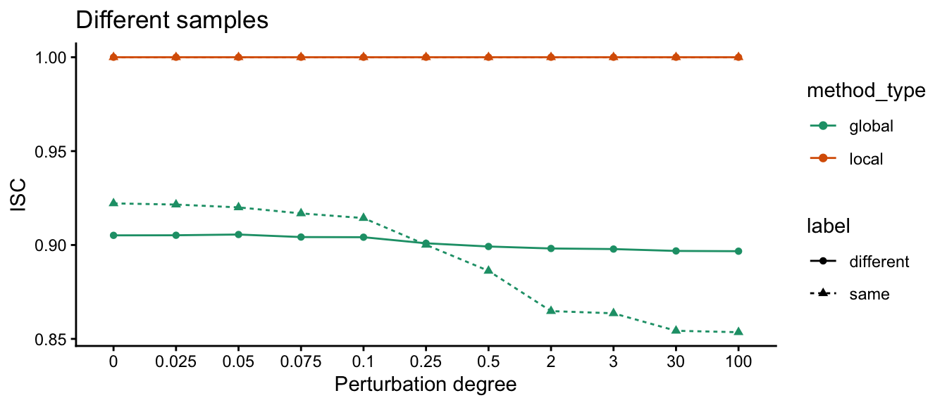
# show pca and RCM plots as well
pca_rcm <- merge_plots(results,
                       pert_type = "per_sample")
pca_rcm
#> $different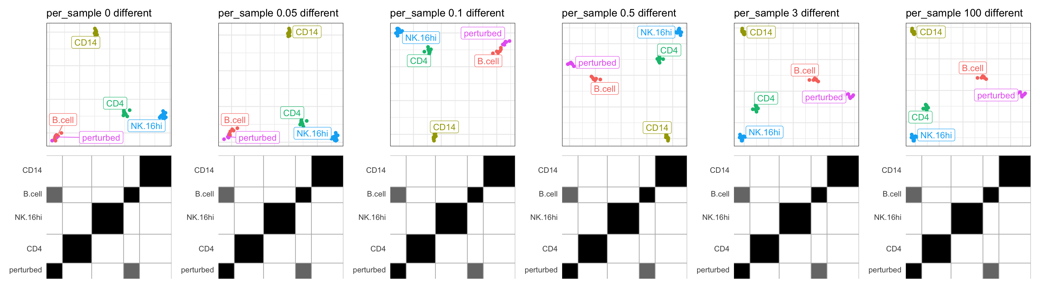
#>
#> $same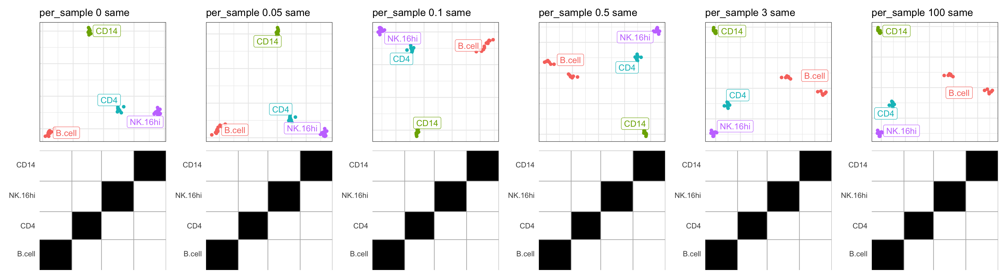
6.2 Perturbing gene expression in 50% of cells within each sample
In this scenario, B_cell is perturbed by randomly selecting half of the cells in each sample and progressively changing their expression profiles.
When the same label is retained, increasing perturbation introduces heterogeneity within one annotation group, which is mainly reflected by a decline in global ISC. When different labels are assigned, local ISC starts low at weak perturbation (indicating over-splitting of a mostly shared state) and then rises as perturbation increases, consistent with the emergence of two truly distinct states.
pert_type <- "50% each sample"
# evolution line
line_pl <-  df %>%
  filter(perturbation_type == pert_type) %>%
   ggplot(aes(noise, measure, color = method_type)) +
   geom_point(aes(shape = label)) +
   geom_line(aes(group = isc,
                 linetype = label)) +
   scale_color_manual(values = cols) +
   labs(y = "ISC",
        x = "Perturbation degree",
        title = pert_type) +
   theme_classic()
line_pl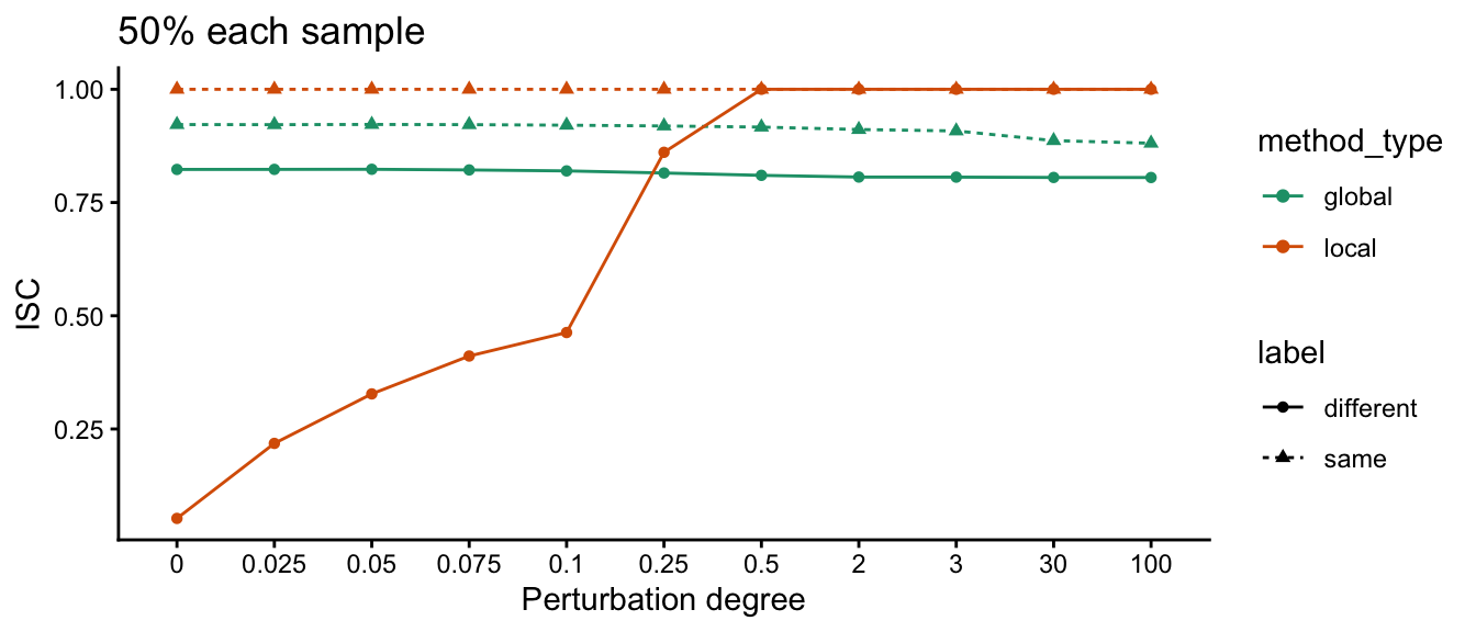
# show pca and RCM plots as well
pca_rcm <- merge_plots(results,
                       pert_type = "same_sample")
pca_rcm
#> $different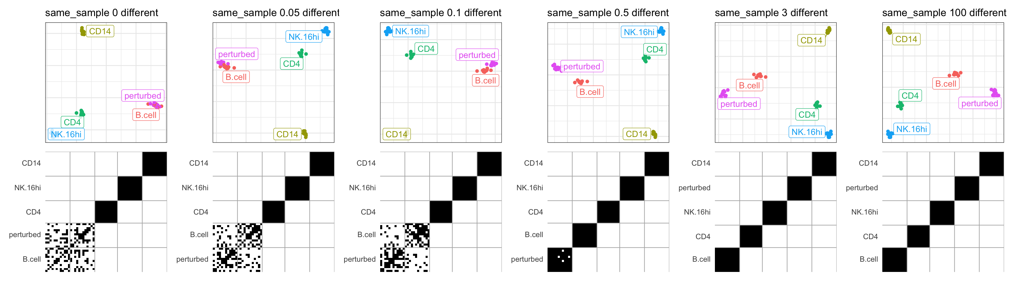
#>
#> $same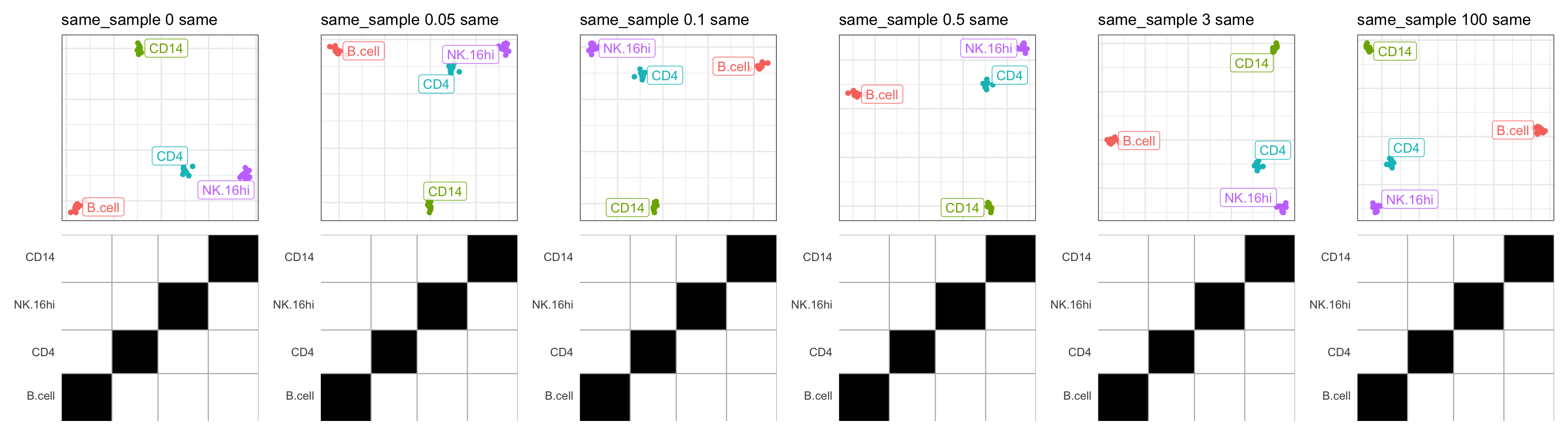
6.3 Perturbing gene expression in either 75% or 25% of cells within each sample
In this scenario, B_cell is perturbed by selecting 75% of cells in some samples and 25% in others. This setup simulates an annotated cell type composed of sub-states present at different proportions across individuals.
The pattern is similar to the 50%-per-sample scenario: global ISC declines under shared labeling as within-label heterogeneity grows, while local ISC improves under refined labeling once perturbation is strong enough to justify a split.
pert_type <- "25% | 75% of each sample"
# evolution line
line_pl <-  df %>%
  filter(perturbation_type == pert_type) %>%
   ggplot(aes(noise, measure, color = method_type)) +
   geom_point(aes(shape = label)) +
   geom_line(aes(group = isc,
                 linetype = label)) +
   scale_color_manual(values = cols) +
   labs(y = "ISC",
        x = "Perturbation degree",
        title = pert_type) +
   theme_classic()
line_pl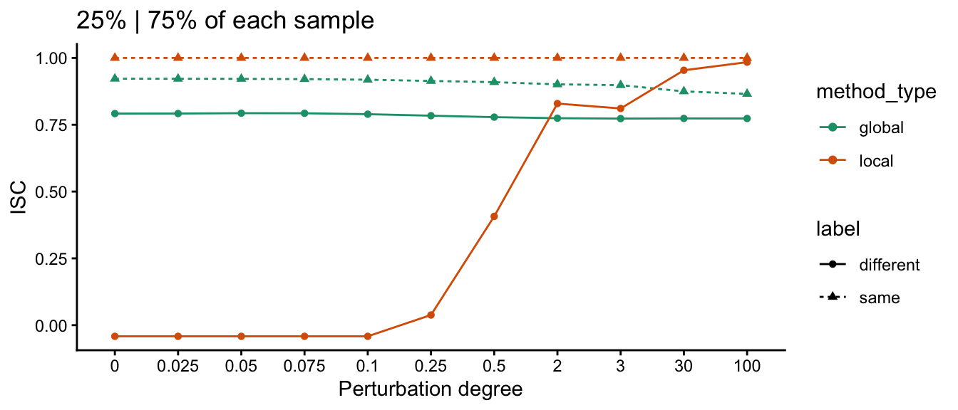
# show pca and RCM plots as well
pca_rcm <- merge_plots(results,
                       pert_type = "different_sample")
pca_rcm
#> $different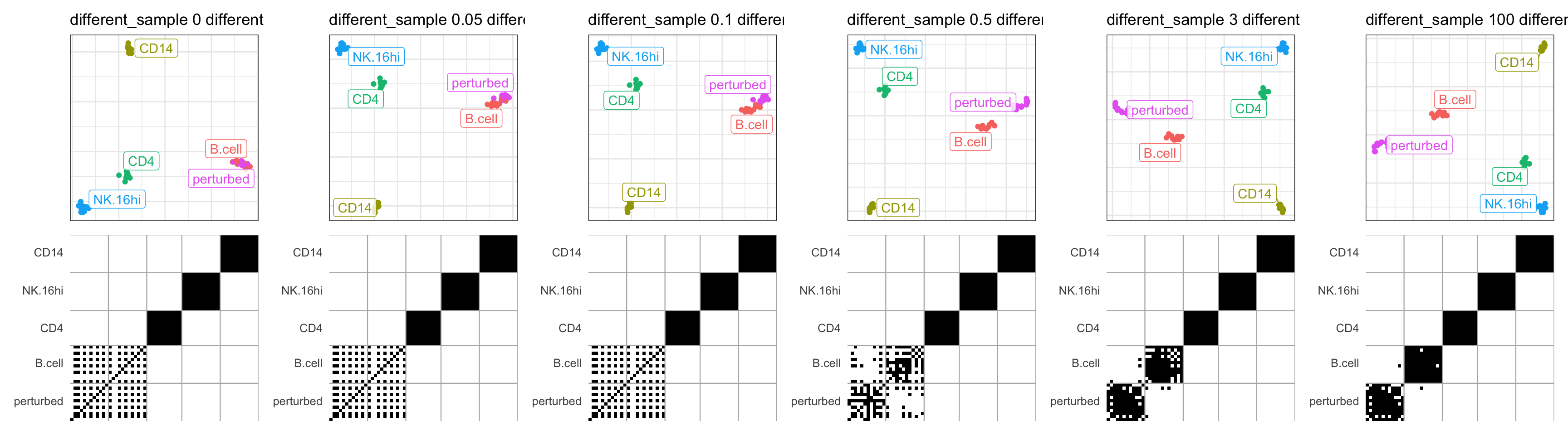
#>
#> $same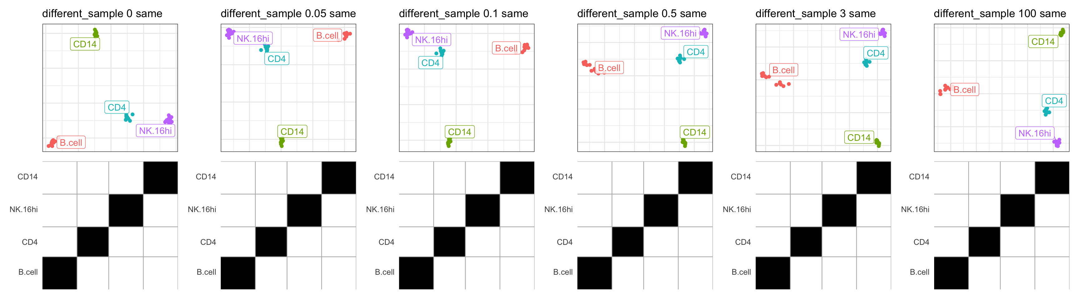
7 Interpretation
These semi-synthetic experiments show complementary behavior of local and global ISC under controlled perturbations:
- Global ISC is most informative when heterogeneous states are forced under the same label. As perturbation intensity increases, global ISC decreases, indicating that a single label no longer captures a coherent cross-sample population.
- Local ISC is most informative for label validity after splitting. When two labels are assigned but perturbation is weak, local ISC remains low (unsupported split). As perturbation increases, local ISC rises, supporting a biologically meaningful subdivision.
- Together, these metrics provide a practical refinement rule: low global ISC under shared labels suggests potential under-partitioning, whereas low local ISC under refined labels indicates over-partitioning.
- The consistency patterns are robust across different perturbation designs (sample-wise, equal within-sample, and unequal within-sample), supporting ISC as a stable diagnostic for annotation granularity.
8 Session information
sessionInfo()
#> R version 4.6.0 alpha (2026-03-31 r89754)
#> Platform: aarch64-apple-darwin23
#> Running under: macOS Tahoe 26.5.1
#>
#> Matrix products: default
#> BLAS:   /Library/Frameworks/R.framework/Versions/4.6/Resources/lib/libRblas.0.dylib
#> LAPACK: /Library/Frameworks/R.framework/Versions/4.6/Resources/lib/libRlapack.dylib;  LAPACK version 3.12.1
#>
#> locale:
#> [1] en_US.UTF-8/en_US.UTF-8/en_US.UTF-8/C/en_US.UTF-8/en_US.UTF-8
#>
#> time zone: Europe/Zurich
#> tzcode source: internal
#>
#> attached base packages:
#> [1] stats     graphics  grDevices datasets  utils     methods   base
#>
#> other attached packages:
#> [1] patchwork_1.3.2  ggplot2_4.0.3    tidyr_1.3.2      dplyr_1.2.1
#> [5] Matrix_1.7-5     scTypeEval_1.0.0
#>
#> loaded via a namespace (and not attached):
#>  [1] SummarizedExperiment_1.42.0 gtable_0.3.6
#>  [3] xfun_0.60                   htmlwidgets_1.6.4
#>  [5] ggrepel_0.9.8               Biobase_2.72.0
#>  [7] lattice_0.22-9              vctrs_0.7.3
#>  [9] tools_4.6.0                 generics_0.1.4
#> [11] stats4_4.6.0                parallel_4.6.0
#> [13] tibble_3.3.1                cluster_2.1.8.2
#> [15] pkgconfig_2.0.3             BiocNeighbors_2.6.0
#> [17] data.table_1.18.4           RColorBrewer_1.1-3
#> [19] dqrng_0.4.1                 S7_0.2.2
#> [21] S4Vectors_0.50.1            lifecycle_1.0.5
#> [23] compiler_4.6.0              farver_2.1.2
#> [25] statmod_1.5.2               bluster_1.22.0
#> [27] Seqinfo_1.2.0               codetools_0.2-20
#> [29] htmltools_0.5.9             yaml_2.3.12
#> [31] pillar_1.11.1               BiocParallel_1.46.0
#> [33] SingleCellExperiment_1.34.0 limma_3.68.4
#> [35] DelayedArray_0.38.2         abind_1.4-8
#> [37] metapod_1.20.0              locfit_1.5-9.12
#> [39] rsvd_1.0.5                  tidyselect_1.2.1
#> [41] digest_0.6.39               BiocSingular_1.28.0
#> [43] purrr_1.2.2                 labeling_0.4.3
#> [45] fastmap_1.2.0               grid_4.6.0
#> [47] cli_3.6.6                   SparseArray_1.12.2
#> [49] magrittr_2.0.5              S4Arrays_1.12.0
#> [51] edgeR_4.10.1                withr_3.0.3
#> [53] scales_1.4.0                rmarkdown_2.31
#> [55] XVector_0.52.0              matrixStats_1.5.0
#> [57] igraph_2.3.3                otel_0.2.0
#> [59] scran_1.40.0                ScaledMatrix_1.20.0
#> [61] beachmat_2.28.0             evaluate_1.0.5
#> [63] knitr_1.51                  GenomicRanges_1.64.0
#> [65] IRanges_2.46.0              irlba_2.3.7
#> [67] rlang_1.3.0                 Rcpp_1.1.2
#> [69] scuttle_1.22.0              glue_1.8.1
#> [71] renv_1.2.3                  BiocGenerics_0.58.1
#> [73] rstudioapi_0.19.0           jsonlite_2.0.0
#> [75] R6_2.6.1                    MatrixGenerics_1.24.0