Getting Started

Author

Affiliation

Josep Garnica

University of Geneva

Published

July 16, 2026

Overview

This quick start guide demonstrates the essential steps for evaluating cell type annotations using scTypeEval. For a comprehensive tutorial, see the main vignette.

library(scTypeEval)

Minimal Workflow

From a Count Matrix

library(Matrix)

# Generate example data
set.seed(123)
counts <- Matrix(rpois(50000, 5), nrow=500, ncol=100, sparse=TRUE)
rownames(counts) <- paste0("Gene", seq_len(500))
colnames(counts) <- paste0("Cell", seq_len(100))

metadata <- data.frame(
  celltype = rep(c("TypeA", "TypeB", "TypeC", "TypeD"), each=25),
  sample = rep(paste0("S", seq_len(5)), times=20),
  row.names = colnames(counts)
)

# Create object
sceval <- create_scTypeEval(matrix=counts, metadata=metadata)

# Process data
sceval <- run_processing_data(
  sceval,
  ident = "celltype",
  sample = "sample",
  min_samples = 3,
  min_cells = 5
)
#> # Processing data for single-cell ...
#>    Transforming and filtering count matrix...
#>    Normalizing count matrix via Log1p...
#> # Processing data for pseudobulk ...
#>    Transforming and filtering count matrix...
#>    Normalizing count matrix via Log1p...

# Identify features
sceval <- run_hvg(sceval,
                  var_method = "basic",
                  ngenes = 1000)
#> Not using black gene list
#> Computing HVG...

# Run PCA
sceval <- run_pca(sceval, ndim = 20)
#> 
#> Using HVG gene list.
#> Not using black gene list
#> # Computing PCA data for single-cell ...
#>    Filtering gene list...
#>    Filtering empty rows and cols...
#>    Computing PCA space...
#>    > Returning 20 dimensions for PCA
#> # Computing PCA data for pseudobulk ...
#>    Filtering gene list...
#>    Filtering empty rows and cols...
#>    Computing PCA space...
#>    > Returning 19 dimensions for PCA

# Compute dissimilarity
sceval <- run_dissimilarity(
  sceval,
  method = "Pseudobulk:Euclidean",
  reduction = TRUE
)
#>    Running distance for euclidean...

# Get consistency
results <- get_consistency(
  sceval,
  dissimilarity_slot = "Pseudobulk:Euclidean",
  consistency_metric = "silhouette"
)
#> Computing internal validation metrics for Pseudobulk:Euclidean ...
print(results)
#>       celltype      measure consistency_metric dissimilarity_method    ident
#> TypeA    TypeA  0.009929989         silhouette Pseudobulk:Euclidean celltype
#> TypeB    TypeB -0.011988536         silhouette Pseudobulk:Euclidean celltype
#> TypeC    TypeC -0.005448364         silhouette Pseudobulk:Euclidean celltype
#> TypeD    TypeD -0.020708784         silhouette Pseudobulk:Euclidean celltype

From a Seurat Object

library(Seurat)

# Create Seurat object with example data generated earlier
seurat_obj <- Seurat::CreateSeuratObject(
  counts = counts,
  meta.data = metadata
)

sceval_seurat <- create_scTypeEval(seurat_obj)

# Continue with standard workflow

From a SingleCellExperiment Object

library(SingleCellExperiment)

# Create SCE object with example data generated earlier
sce <- SingleCellExperiment::SingleCellExperiment(
  assays = list(counts = counts),
  colData = metadata
)

sceval_sce <- create_scTypeEval(sce)

# Continue with workflow as above

Common Use Cases

Compare Multiple Dissimilarity Methods

# Compute different dissimilarity methods
sceval <- run_dissimilarity(
  sceval,
  method = "Pseudobulk:Euclidean",
  reduction = TRUE
)
#>    Running distance for euclidean...
sceval <- run_dissimilarity(
  sceval,
  method = "Pseudobulk:Cosine",
  reduction = TRUE
)
#>    Running distance for cosine...
sceval <- run_dissimilarity(
  sceval,
  method = "WasserStein",
  reduction = TRUE
)
#> Splitting matrices...
#> Computing pairwise WasserStein distance...

# Compare consistency across methods
dissimilarity_methods <- c("Pseudobulk:Euclidean",
                           "Pseudobulk:Cosine",
                           "WasserStein")
results_df <- 
  get_consistency(
    sceval,
    dissimilarity_slot = dissimilarity_methods, # compute for multiple dissimilarities
    consistency_metric = "silhouette"
  )
#> Computing internal validation metrics for Pseudobulk:Euclidean ...
#> Computing internal validation metrics for Pseudobulk:Cosine ...
#> Computing internal validation metrics for WasserStein ...

results_df
#>        celltype      measure consistency_metric dissimilarity_method    ident
#> TypeA     TypeA  0.009929989         silhouette Pseudobulk:Euclidean celltype
#> TypeB     TypeB -0.011988536         silhouette Pseudobulk:Euclidean celltype
#> TypeC     TypeC -0.005448364         silhouette Pseudobulk:Euclidean celltype
#> TypeD     TypeD -0.020708784         silhouette Pseudobulk:Euclidean celltype
#> TypeA1    TypeA -0.003214443         silhouette    Pseudobulk:Cosine celltype
#> TypeB1    TypeB -0.002765134         silhouette    Pseudobulk:Cosine celltype
#> TypeC1    TypeC -0.013348235         silhouette    Pseudobulk:Cosine celltype
#> TypeD1    TypeD -0.022767009         silhouette    Pseudobulk:Cosine celltype
#> TypeA2    TypeA  0.034467020         silhouette          WasserStein celltype
#> TypeB2    TypeB -0.026486747         silhouette          WasserStein celltype
#> TypeC2    TypeC -0.026581239         silhouette          WasserStein celltype
#> TypeD2    TypeD -0.043528190         silhouette          WasserStein celltype

Evaluate Multiple Consistency Metrics

# Compute multiple consistency metrics
consistency_metrics <- c("silhouette",
                         "NeighborhoodPurity",
                         "Average_similarity")

all_metrics <- 
  get_consistency(
    sceval,
    dissimilarity_slot = "Pseudobulk:Euclidean",
    consistency_metric = consistency_metrics
  )
#> Computing internal validation metrics for Pseudobulk:Euclidean ...

all_metrics
#>        celltype      measure consistency_metric dissimilarity_method    ident
#> TypeA     TypeA  0.009929989         silhouette Pseudobulk:Euclidean celltype
#> TypeB     TypeB -0.011988536         silhouette Pseudobulk:Euclidean celltype
#> TypeC     TypeC -0.005448364         silhouette Pseudobulk:Euclidean celltype
#> TypeD     TypeD -0.020708784         silhouette Pseudobulk:Euclidean celltype
#> TypeA1    TypeA  0.320000000 NeighborhoodPurity Pseudobulk:Euclidean celltype
#> TypeB1    TypeB  0.240000000 NeighborhoodPurity Pseudobulk:Euclidean celltype
#> TypeC1    TypeC  0.240000000 NeighborhoodPurity Pseudobulk:Euclidean celltype
#> TypeD1    TypeD  0.200000000 NeighborhoodPurity Pseudobulk:Euclidean celltype
#> TypeA2    TypeA  0.504617271 Average_similarity Pseudobulk:Euclidean celltype
#> TypeB2    TypeB  0.500755570 Average_similarity Pseudobulk:Euclidean celltype
#> TypeC2    TypeC  0.501285885 Average_similarity Pseudobulk:Euclidean celltype
#> TypeD2    TypeD  0.498308342 Average_similarity Pseudobulk:Euclidean celltype

Visualize Results

# Heatmap of dissimilarities
plot_heatmap(
  sceval,
  dissimilarity_slot = "Pseudobulk:Euclidean",
  sort_consistency = "silhouette"
)
#> Computing consistency metric for silhouette.
#> Consistency computed.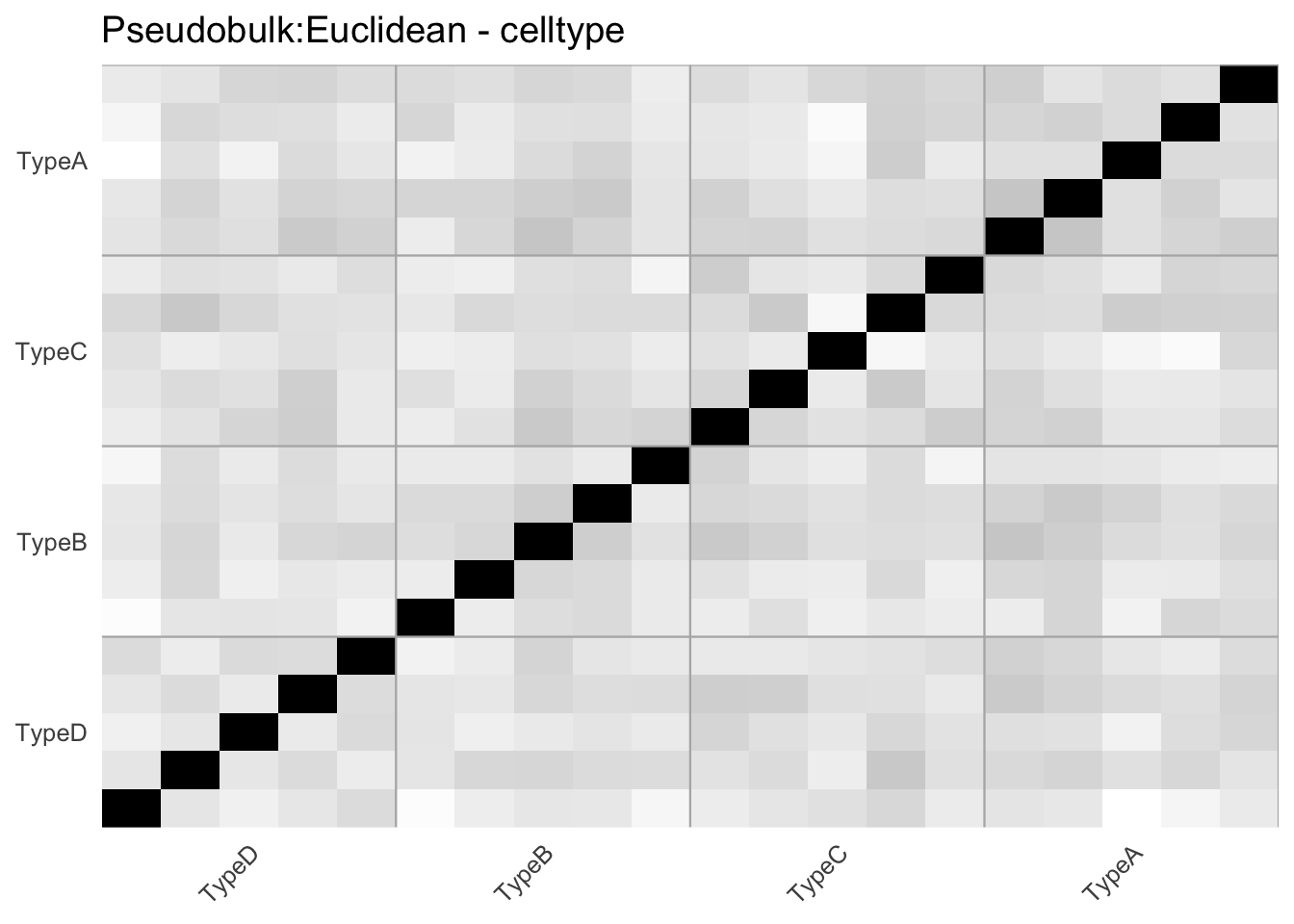


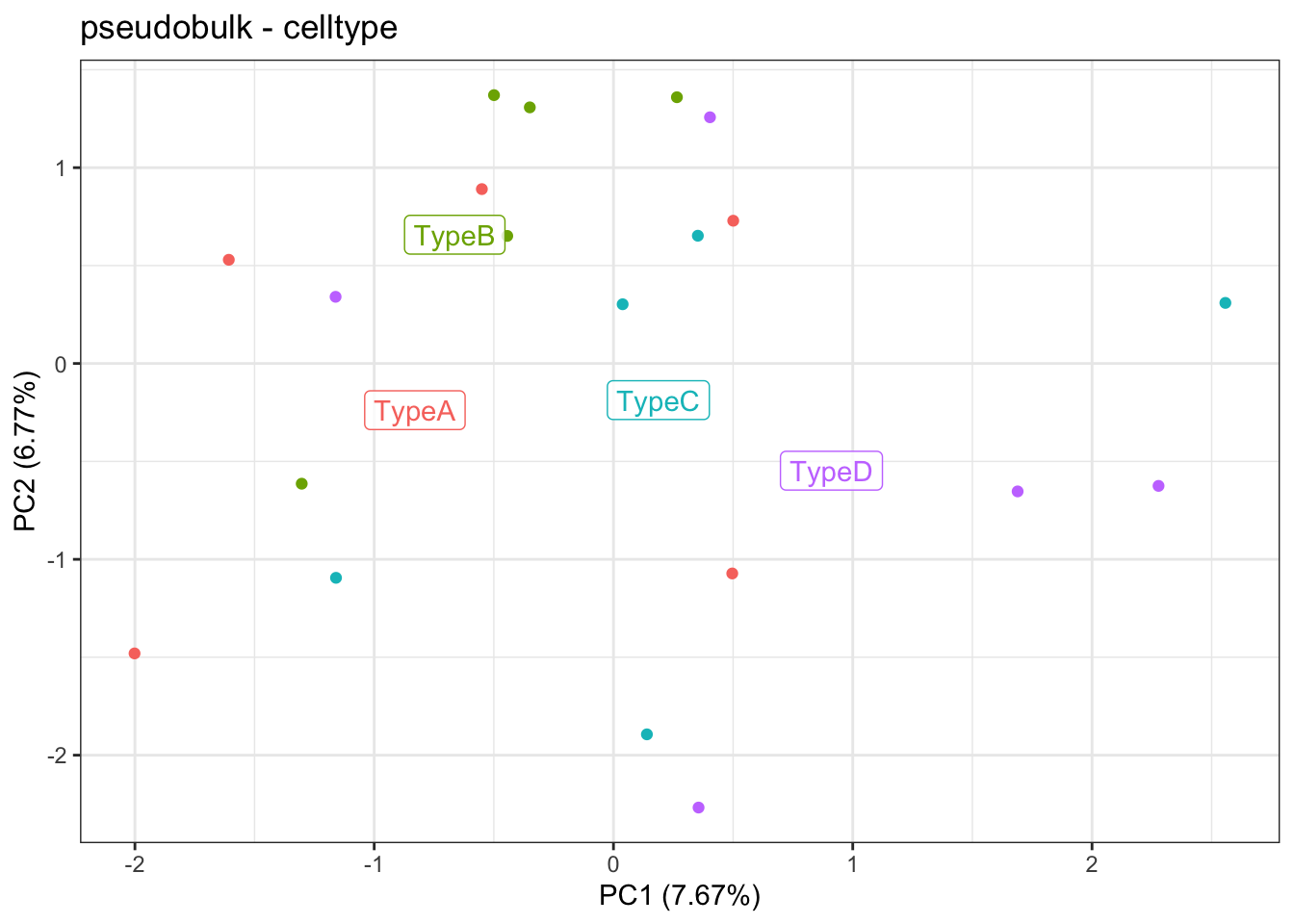
# Pseudobulk PCA per sample & cell type
plot_pca(
  sceval,
  reduction_slot = "pseudobulk"
)

Using Marker Genes Instead of HVGs

# Identify cell type markers
sceval <- run_gene_markers(
  sceval,
  method = "scran.findMarkers",
  ngenes_celltype = 50
)
#> Not using black gene list
#> Computing cell type markers for celltype...

# Use markers for dissimilarity calculation
sceval <- run_dissimilarity(
  sceval,
  method = "Pseudobulk:Euclidean",
  gene_list = "scran.findMarkers", # gene list recently added
  reduction = FALSE
)
#> 
#> Using scran.findMarkers gene list.
#> Not using black gene list
#>    Filtering gene list...
#>    Filtering empty rows and cols...
#>    Running distance for euclidean...

Focus on Specific Gene Sets

# Add custom gene list
immune_genes <- c("CD3D", "CD4", "CD8A", "CD19", "CD14", "NCAM1")
sceval <- add_gene_list(
  sceval,
  gene_list = list("immune_markers" = immune_genes) # add a named list
)

# Run analysis on custom genes
sceval <- run_dissimilarity(
  sceval,
  method = "Pseudobulk:Euclidean",
  gene_list = "immune_markers" # name of the list to use
)
#>    Running distance for euclidean...

Interpreting Results

What Low Scores Mean

Low consistency scores may indicate:

Ambiguous cell type boundaries between related types
Heterogeneous populations needing refinement
Annotation inconsistencies across samples

Next Steps for Low-Scoring Cell Types

Visualize using plot_heatmap() or plot_pca() to identify problematic samples
Investigate biological differences (e.g., disease vs. healthy)
Refine annotations by splitting or merging cell types

Available Methods and Metrics

Dissimilarity Methods

Pseudobulk:Euclidean - Euclidean distance on pseudobulk profiles
Pseudobulk:Cosine - Cosine distance on pseudobulk profiles
Pseudobulk:Pearson - Pearson correlation distance on pseudobulk profiles
WasserStein - Wasserstein distance between cell distributions
recip_classif:Match - Reciprocal classification matching
recip_classif:Score - Reciprocal classification scoring

Consistency Metrics

silhouette - Standard silhouette coefficient
2label_silhouette - Two-label silhouette variant
NeighborhoodPurity - K-nearest neighbor purity
ward_PropMatch - Ward clustering proportion match
Orbital_medoid - Medoid-based orbital metric
Average_similarity - Average within-group similarity

Tips and Best Practices

Always use multiple samples (minimum 3-5 per cell type)
Compare different methods - no single method is perfect
Use PCA for speed - similar results, much faster
Start with HVGs - then try marker genes if needed
Check sample sizes - ensure adequate cells per type per sample
Interpret in context - consider biological heterogeneity

Getting Help

GitHub: https://github.com/carmonalab/scTypeEval
Issues: https://github.com/carmonalab/scTypeEval/issues
Main vignette: browseVignettes("scTypeEval")

Session Info

sessionInfo()
#> R version 4.6.0 alpha (2026-03-31 r89754)
#> Platform: aarch64-apple-darwin23
#> Running under: macOS Tahoe 26.5.1
#> 
#> Matrix products: default
#> BLAS:   /Library/Frameworks/R.framework/Versions/4.6/Resources/lib/libRblas.0.dylib 
#> LAPACK: /Library/Frameworks/R.framework/Versions/4.6/Resources/lib/libRlapack.dylib;  LAPACK version 3.12.1
#> 
#> locale:
#> [1] en_US.UTF-8/en_US.UTF-8/en_US.UTF-8/C/en_US.UTF-8/en_US.UTF-8
#> 
#> time zone: Europe/Zurich
#> tzcode source: internal
#> 
#> attached base packages:
#> [1] stats4    stats     graphics  grDevices datasets  utils     methods  
#> [8] base     
#> 
#> other attached packages:
#>  [1] SingleCellExperiment_1.34.0 SummarizedExperiment_1.42.0
#>  [3] Biobase_2.72.0              GenomicRanges_1.64.0       
#>  [5] Seqinfo_1.2.0               IRanges_2.46.0             
#>  [7] S4Vectors_0.50.1            BiocGenerics_0.58.1        
#>  [9] generics_0.1.4              MatrixGenerics_1.24.0      
#> [11] matrixStats_1.5.0           Seurat_5.5.1               
#> [13] SeuratObject_5.4.0          sp_2.2-1                   
#> [15] Matrix_1.7-5                scTypeEval_1.0.0           
#> 
#> loaded via a namespace (and not attached):
#>   [1] RColorBrewer_1.1-3     jsonlite_2.0.0         magrittr_2.0.5        
#>   [4] spatstat.utils_3.2-3   farver_2.1.2           rmarkdown_2.31        
#>   [7] vctrs_0.7.3            ROCR_1.0-12            spatstat.explore_3.8-1
#>  [10] htmltools_0.5.9        S4Arrays_1.12.0        BiocNeighbors_2.6.0   
#>  [13] SparseArray_1.12.2     sctransform_0.4.3      parallelly_1.48.0     
#>  [16] KernSmooth_2.23-26     htmlwidgets_1.6.4      ica_1.0-3             
#>  [19] plyr_1.8.9             plotly_4.12.0          zoo_1.8-15            
#>  [22] igraph_2.3.3           mime_0.13              lifecycle_1.0.5       
#>  [25] pkgconfig_2.0.3        rsvd_1.0.5             R6_2.6.1              
#>  [28] fastmap_1.2.0          fitdistrplus_1.2-6     future_1.70.0         
#>  [31] shiny_1.14.0           digest_0.6.39          patchwork_1.3.2       
#>  [34] tensor_1.5.1           dqrng_0.4.1            RSpectra_0.16-2       
#>  [37] irlba_2.3.7            beachmat_2.28.0        labeling_0.4.3        
#>  [40] progressr_1.0.0        spatstat.sparse_3.2-0  httr_1.4.8            
#>  [43] polyclip_1.10-7        abind_1.4-8            compiler_4.6.0        
#>  [46] withr_3.0.3            S7_0.2.2               BiocParallel_1.46.0   
#>  [49] fastDummies_1.7.6      MASS_7.3-65            DelayedArray_0.38.2   
#>  [52] bluster_1.22.0         tools_4.6.0            lmtest_0.9-40         
#>  [55] otel_0.2.0             httpuv_1.6.17          future.apply_1.20.2   
#>  [58] goftest_1.2-3          glue_1.8.1             nlme_3.1-169          
#>  [61] promises_1.5.0         grid_4.6.0             Rtsne_0.17            
#>  [64] cluster_2.1.8.2        reshape2_1.4.5         gtable_0.3.6          
#>  [67] spatstat.data_3.1-9    tidyr_1.3.2            data.table_1.18.4     
#>  [70] metapod_1.20.0         ScaledMatrix_1.20.0    BiocSingular_1.28.0   
#>  [73] XVector_0.52.0         spatstat.geom_3.8-1    RcppAnnoy_0.0.23      
#>  [76] ggrepel_0.9.8          RANN_2.6.2             pillar_1.11.1         
#>  [79] stringr_1.6.0          limma_3.68.4           spam_2.11-4           
#>  [82] RcppHNSW_0.7.0         later_1.4.8            splines_4.6.0         
#>  [85] dplyr_1.2.1            lattice_0.22-9         renv_1.2.3            
#>  [88] survival_3.8-6         deldir_2.0-4           tidyselect_1.2.1      
#>  [91] locfit_1.5-9.12        scuttle_1.22.0         miniUI_0.1.2          
#>  [94] pbapply_1.7-4          transport_0.15-4       knitr_1.51            
#>  [97] gridExtra_2.3.1        edgeR_4.10.1           scattermore_1.2       
#> [100] xfun_0.60              statmod_1.5.2          stringi_1.8.7         
#> [103] lazyeval_0.2.3         yaml_2.3.12            evaluate_1.0.5        
#> [106] codetools_0.2-20       tibble_3.3.1           cli_3.6.6             
#> [109] uwot_0.2.4             xtable_1.8-8           reticulate_1.46.0     
#> [112] Rcpp_1.1.2             globals_0.19.1         spatstat.random_3.5-0 
#> [115] png_0.1-9              spatstat.univar_3.2-0  parallel_4.6.0        
#> [118] ggplot2_4.0.3          dotCall64_1.2          scran_1.40.0          
#> [121] listenv_1.0.0          viridisLite_0.4.3      scales_1.4.0          
#> [124] ggridges_0.5.7         purrr_1.2.2            rlang_1.3.0           
#> [127] cowplot_1.2.0