Human Lung Cell Atlas (HLCA) reannotation with ISC

Author
Affiliation

Josep Garnica

University of Geneva

Published

July 16, 2026

1 Introduction

This case study reproduces the ISC-guided annotation refinement strategy presented for the Human Lung Cell Atlas (HLCA) in Figure 6 of the scTypeEval publication. This tutorial walks through each step of the scTypeEval workflow, comparing the original and refined annotation frameworks. The objective is to illustrate how inter-sample consistency (ISC) can be used to identify annotation levels that are robust across individuals and to guide biologically meaningful annotation refinement.

2 Dataset description

This tutorial uses the Human Lung Cell Atlas (HLCA) published by Sikkema et al., 2023, a large-scale integrated single-cell reference atlas of the human respiratory tract. The HLCA core contains healthy lung tissue from 107 individuals collected across multiple studies and includes consensus manual cell type annotations curated independently by six experts.

For this case study, raw gene expression counts and metadata are downloaded from Zenodo and cached locally. This core dataset from HLCA can also be found at CELLxGENE

Although the published HLCA provides an integrated low-dimensional embedding generated using scANVI, the analyses in this tutorial start from the raw count matrix. This allows the complete preprocessing, feature selection, dimensionality reduction, dissimilarity computation, and ISC evaluation workflow to be reproduced using scTypeEval.

3 Download data

hlca_url <- paste0(
  "https://zenodo.org/records/18921437/files/",
  "Sikkema_2023_37291214_b351804c-293e-4aeb-9c4c-043db67f4540.rds?download=1"
)

cache_dir <- file.path("cache")
dir.create(cache_dir, recursive = TRUE, showWarnings = FALSE)

dataset_file <- file.path(
  cache_dir,
  "Sikkema_2023_37291214_b351804c-293e-4aeb-9c4c-043db67f4540.rds"
)

if (!file.exists(dataset_file)) {
  old_timeout <- getOption("timeout")
  on.exit(options(timeout = old_timeout), add = TRUE)
  options(timeout = 99999)
  utils::download.file(hlca_url, dataset_file, mode = "wb")
}

dataset_file
[1] "cache/Sikkema_2023_37291214_b351804c-293e-4aeb-9c4c-043db67f4540.rds"

4 Load packages and constants

library(dplyr)
library(tidyr)
library(ggplot2)
library(scTypeEval)
library(Seurat)
theme_set(theme_bw(base_size = 12))
# Blacklisted genes that are inherently variable across samples
# and should be excluded from ISC (scTypeEval) computations
data(black_list)
blacklist_genes <- c(black_list$TCR, black_list$Immunoglobulins, black_list$Ygenes)
# These are the local and global ISC thresholds empirically described in the manuscript (Fig. 5)
q_local <- 0.4467538
q_global <- 0.7443436

5 Load HLCA object

6 Downsample dataset

For this tutorial, we downsample the dataset to a maximum of 200 cells per cell type and sample combination. This makes the analysis lighter while preserving cell type and sample representation.

obj <- readRDS(dataset_file)
obj$Sample_annot <- paste(obj$sample, obj$cell_type)
Idents(obj) <- "Sample_annot"
# Set seed for downsampling
# we'll keep max 200 cells per cell type and sample
set.seed(22)
obj2 <- subset(obj, downsample = 200)
dim(obj2)
[1]  27957 198015
# split into counts and metadata
counts <- LayerData(obj2, layer = "counts")
metadata <- obj2@meta.data
# for metadata keep only columns that will be used later
col_md_keep <- c("cell_type", # main annotation framework
                 "ann_level_4", # information of lineage of cell types
                 "sample", # sample or origin
                 "donor_id",
                 "dataset", # batch id
                 "tissue" # tissue of origin
                 )
metadata <- metadata %>% 
  select(all_of(col_md_keep))

6.1 Dataset specifics

The HLCA core dataset contains:

  • 584K cells - subsampled into 198K
  • 166 samples (sample)
  • 107 donors (donor_id)
  • 14 different datasets of origin or batches (dataset)
  • 3 different tissues of origin within the respiratory tract (tissue): lung parenchyma, respiratory airway, and nose
  • 50 cell types in their main annotation framework (cell_type)

7 ISC on baseline annotations

We will explore ISC on the default annotation of the atlas: cell_type.

7.1 Create scTypeEval object

sceval_original <- create_scTypeEval(
  matrix = counts,
  metadata = metadata
)

7.2 Process data and obtain HVG

sceval_original <- run_processing_data(
  scTypeEval = sceval_original,
  ident = "cell_type", # default annotation of lung atlas
  sample = "sample",
  min_samples = 5,
  min_cells = 10,
  verbose = FALSE
)
sceval_original <- run_hvg(
  scTypeEval = sceval_original,
  var_method = "scran",
  ngenes = 2000,
  sample = TRUE,
  aggregation = "single-cell",
  black_list = blacklist_genes,
  ncores = 6,
  verbose = FALSE
)

7.3 Add PCA embeddings (run_pca)

# remove data from single-cell grouping as we don't need it
sceval_original@data$`single-cell` <- NULL
set.seed(22)
sceval_original <- run_pca(
  scTypeEval = sceval_original,
  ndim = 30,
  verbose = FALSE
)
# Visualize PCA by cell type and sample groups
plot_pca(sceval_original)

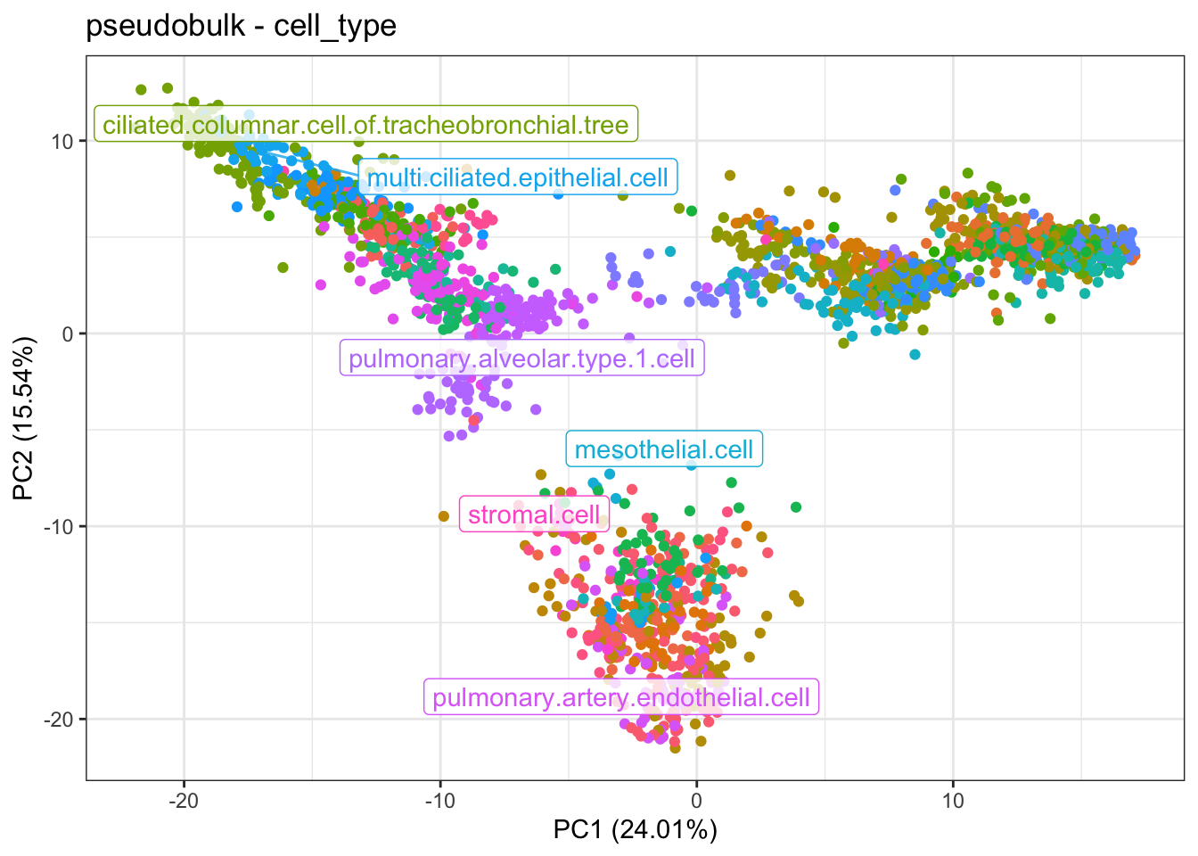
Here we can see the 3 main cell type families in 3 major group of cell types/samples: 1) immune cells, epithelial-respiratory cells, and stromal/endothelial cells.

7.4 Compute dissimilarities

Build pairwise distance matrices between all cell types and sample pairs. We will use the dissimilarities that best capture cross-sample variability. For more information, see Benchmarking of ISC metrics.

# recip_classif:Match computation may take few minutes
sceval_original <- run_dissimilarity(
  sceval_original,
  method = "recip_classif:Match",
  reduction = FALSE,
  ncores = 6,
  verbose = FALSE
)
sceval_original <- run_dissimilarity(
  sceval_original,
  method = "Pseudobulk:Cosine",
  reduction = TRUE,
  verbose = FALSE
)

7.5 Compute consistency (get_consistency)

We then compute the consistency metrics from the previously generated distance matrices. We use global and local ISC, defined here as 2-label silhouette + pseudobulk cosine and silhouette + recip_classif:Match, respectively. For additional details, see Benchmarking of ISC metrics.

cons_original_raw <- get_consistency(
  sceval_original,
  dissimilarity_slot = c("recip_classif:Match", "Pseudobulk:Cosine"),
  consistency_metric = c("silhouette", "2label_silhouette")
)
cons_original <- cons_original_raw |>
  mutate(method.type = paste(consistency_metric, dissimilarity_method, sep = " | ")) |>
  filter(method.type %in% c(
    "silhouette | recip_classif:Match",
    "2label_silhouette | Pseudobulk:Cosine"
  )) |>
  mutate(
    metric = factor(
      method.type,
      levels = c(
        "silhouette | recip_classif:Match",
        "2label_silhouette | Pseudobulk:Cosine"
      ),
      labels = c("local", "global")
    )
  ) |>
  select(celltype, metric, measure) |>
  pivot_wider(names_from = metric, values_from = measure) |>
  mutate(integrated_isc = local * global) %>% 
  arrange(integrated_isc)
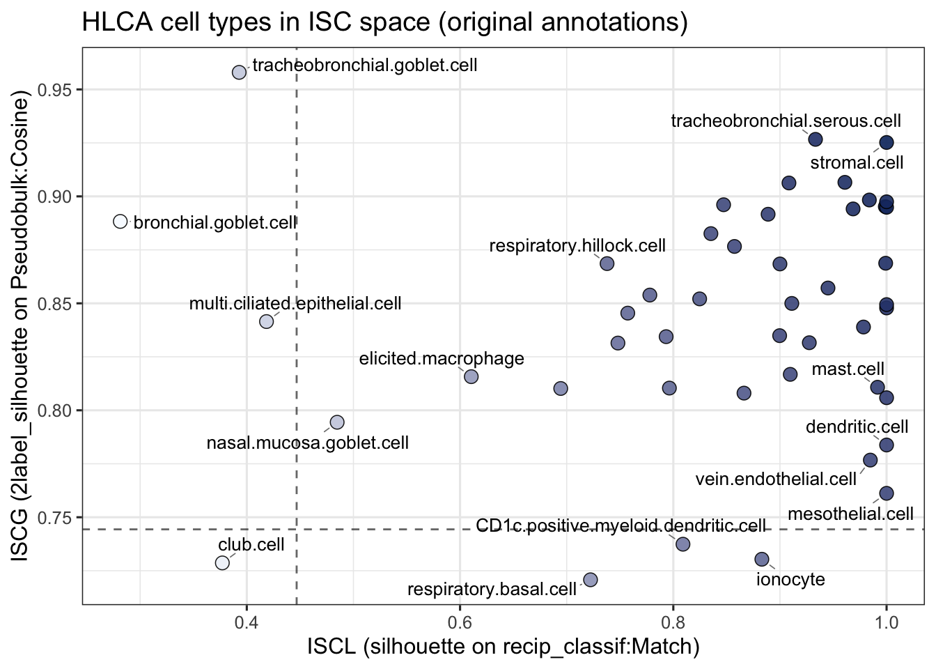
head(cons_original)
# A tibble: 6 × 4
  celltype                       local global integrated_isc
  <chr>                          <dbl>  <dbl>          <dbl>
1 bronchial.goblet.cell          0.281  0.888          0.250
2 club.cell                      0.377  0.729          0.275
3 multi.ciliated.epithelial.cell 0.418  0.841          0.352
4 tracheobronchial.goblet.cell   0.393  0.958          0.376
5 nasal.mucosa.goblet.cell       0.485  0.794          0.385
6 elicited.macrophage            0.611  0.816          0.498

8 Baseline diagnostics

8.1 ISC landscape

cons_original |>
   ggplot(aes(x = local,
             y = global)) +
  # threshold line of figure 5
  geom_vline(
    xintercept = q_local,
    linetype = "dashed",
    linewidth = 0.5,
    alpha = 0.6
  ) +
  geom_hline(
    yintercept = q_global,
    linetype = "dashed",
    linewidth = 0.5,
    alpha = 0.6
  ) +
  # Points
  geom_point(aes(fill = integrated_isc),
             shape = 21,
             size = 3.2,
             stroke = 0.4,
             color = "black",
             alpha = 0.9,
             show.legend = FALSE) +
  
  # Clean blue gradient (Nature-friendly, perceptually smooth)
  scale_fill_gradient(
    low  = "#F7FBFF",
    high = "#08306B"
  ) +
  
  # Repelled labels (better spacing control)
  ggrepel::geom_text_repel(
    aes(label = celltype),
    size = 3.5,
    max.overlaps = 5,
    box.padding = 0.4,
    point.padding = 0.3,
    segment.size = 0.3,
    segment.color = "grey50",
    min.segment.length = 0,
    seed = 22
  ) +
  labs(
    x = "ISCL (silhouette on recip_classif:Match)",
    y = "ISCG (2label_silhouette on Pseudobulk:Cosine)",
    title = "HLCA cell types in ISC space (original annotations)"
  )

The ISC analysis shows that most cell type annotations in the HLCA exhibit high local and global consistency, indicating that these populations are reproducibly identified across individuals. In contrast, a subset of respiratory epithelial populations—including club cells, multiciliated epithelial cells, and bronchial and nasal goblet cells—display substantially lower ISC values. Low local ISC (ISCL) suggests that these populations overlap with neighboring cell states, whereas low global ISC indicates greater transcriptional variability between individuals. These observations suggest that the current annotation framework may not fully capture the underlying biological heterogeneity of these epithelial compartments, making them strong candidates for further refinement.

9 Refine selected epithelial annotations

The presence of low ISC values indicates that these epithelial populations exhibit substantial variability across individuals, but the underlying source of this variability remains unclear. Differences may reflect unresolved biological heterogeneity or limitations of the current annotation framework. Although reclustering low-ISC populations or improving dataset integration are possible approaches, integration methods can also remove meaningful biological variation and reduce interpretability. Therefore, before refining the annotations, we first examine the available metadata to identify whether the observed variability is associated with known biological or technical factors captured in the HLCA dataset.

9.1 Explore metadata

Explore cell type-sample pseudobulk representation of only the cell type with low ISC.

lowISC_cells <- c(
  "bronchial goblet cell",
  "club cell",
  "tracheobronchial goblet cell",
  "multi-ciliated epithelial cell",
  "nasal mucosa goblet cell"
)
sub_meta = metadata %>% 
  filter(cell_type %in% lowISC_cells)
sub_count_matrix = counts[,rownames(sub_meta)]

sc <- create_scTypeEval(matrix = sub_count_matrix,
                        metadata = sub_meta)
sc <- run_processing_data(sc,
                         ident = "cell_type",
                         sample = "sample",
                         verbose = F)
sc <- run_hvg(sc,
              ngenes = 2000,
              ncores = 4, 
              verbose = F,
              black_list = blacklist_genes)
# remove data from single-cell grouping as we don't need it
sc@data$`single-cell` <- NULL
set.seed(22)
sc <- run_pca(sc,
              verbose = F)
col_annot <- data.frame(id = sc@reductions$pseudobulk@group) %>% 
  # this includes <sample_label>_<celltype_label>
  separate(id, sep = "_", into = c("sample", "cell_type"), remove = F) %>% 
  left_join(., sc@metadata %>% 
              distinct(sample, .keep_all = T) %>% 
              mutate(sample = scTypeEval:::purge_label(sample)) %>% 
              select(sample, tissue, dataset),
            by = "sample") %>% 
  tibble::column_to_rownames("id")
pca_list <- lapply(c("cell_type", "tissue"),
                   function(a){
                     sc@reductions$pseudobulk@ident$cell_type <- col_annot[[a]]
                     plot_pca(sc) + ggtitle(a)
                   })
patchwork::wrap_plots(pca_list)

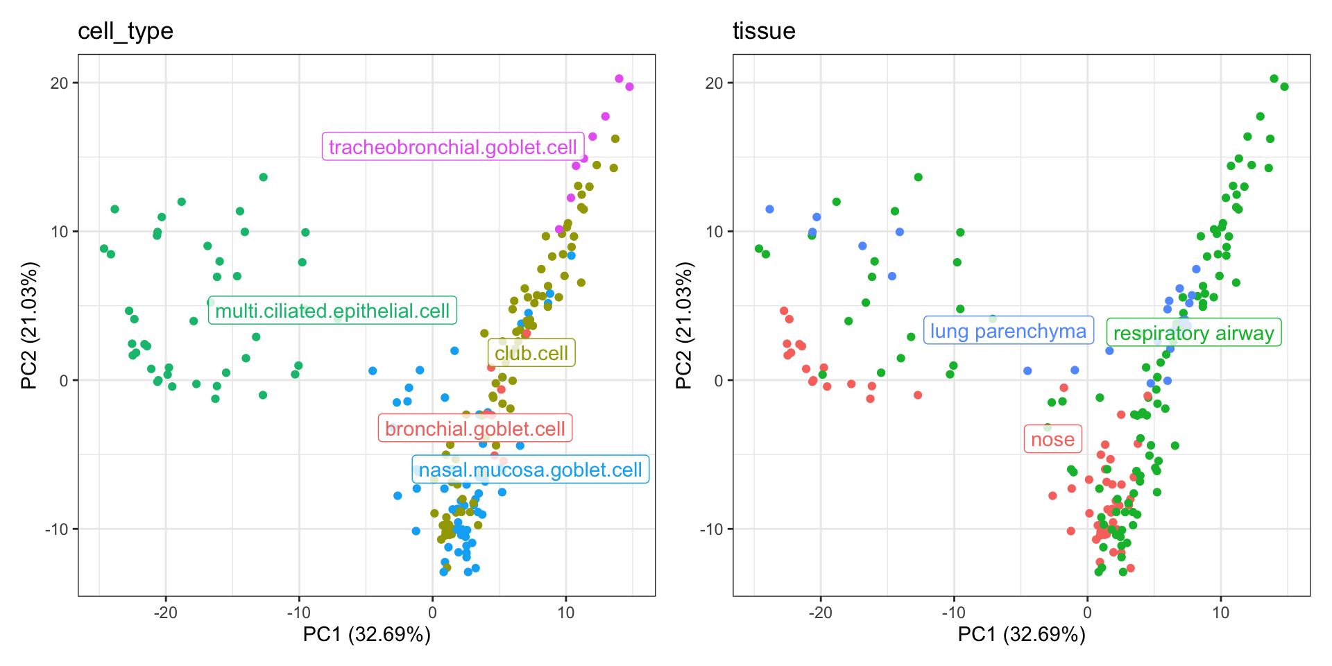
PCA visualization of only low ISC cell types reveals substantial variability across samples, with pseudobulk profiles clustering according to their tissue of origin rather than forming a single homogeneous population. This pattern indicates that tissue-specific transcriptional programs contribute strongly to the observed inter-sample variability, suggesting that the low ISC of these epithelial annotations reflects biologically distinct tissue-associated states rather than annotation inconsistency alone.

9.2 Propose a new annotation for low ISC cell types

Based on the tissue-associated variability observed in the pseudobulk space, we refine low-ISC epithelial annotations by subdividing existing cell types according to their tissue of origin, generating more specific labels that capture airway-, nasal-, and lung-associated epithelial states. Additionally, multi-ciliated epithelial cells can also be classified as Deuterosomal and non-Deuterosomal.

metadata_refined <- metadata |>
    mutate(annot2 = case_when(
    cell_type == "club cell" & tissue == "respiratory airway" ~ "club cell (airway)",
    cell_type == "club cell" & tissue == "nose" ~ "club cell (nasal)",
    cell_type == "club cell" & tissue == "lung parenchyma" ~ "club cell (lung)",
    ##############################################################################
    cell_type == "multi-ciliated epithelial cell" &
      ann_level_4 == "Deuterosomal" ~
      "multi-ciliated epithelial cell (Deuterosomal)",
    cell_type == "multi-ciliated epithelial cell" &
      ann_level_4 != "Deuterosomal" ~
      "multi-ciliated epithelial cell (Non-Deuterosomal)",
    ##############################################################################
    cell_type %in% c("nasal mucosa goblet cell","bronchial goblet cell") &
      tissue == "respiratory airway"~
      NA,
    cell_type %in% c("nasal mucosa goblet cell","bronchial goblet cell") &
      tissue == "nose" ~
      "mucosa goblet cell (nose)",
    cell_type %in% c("nasal mucosa goblet cell","bronchial goblet cell") &
      tissue == "lung parenchyma" ~
      "mucosa goblet cell (lung)",
    ##############################################################################
    cell_type == "tracheobronchial goblet cell" &
      tissue == "respiratory airway" ~
      "tracheobronchial goblet cell(airway)",
    cell_type == "tracheobronchial goblet cell" &
      tissue == "lung parenchyma" ~
      "tracheobronchial goblet cell (lung)",
    cell_type == "tracheobronchial goblet cell" &
      tissue == "nose" ~
      "tracheobronchial goblet cell(nose)",
    TRUE ~ cell_type  # Default case
  )
  )

10 Refined annotations: rerun scTypeEval pipeline

After refining the low-ISC epithelial annotations using tissue-associated information, we rerun the same scTypeEval workflow to evaluate whether the proposed labels improve annotation consistency. According to the ISC-guided refinement principle, successful refinements should increase the consistency metric that identified the original limitation: splitting biologically distinct populations should improve global consistency while preserving local consistency, whereas merging overly similar populations should improve local consistency without reducing global consistency.

10.1 Create object

sceval_refined <- create_scTypeEval(
  matrix = counts,
  metadata = metadata_refined
)

10.2 Run scTypeEval workflow

We will use the newly proposed annotation (annot2) as ident. This keeps the author’s original cell_type labels unchanged except for the low-ISC labels that were refined.

sceval_refined <- run_processing_data(
  scTypeEval = sceval_refined,
  ident = "annot2", # proposed annotation
  sample = "sample",
  min_samples = 5,
  min_cells = 10,
  verbose = FALSE
)
# Obtain HVG for this new annotation
sceval_refined <- run_hvg(
  scTypeEval = sceval_refined,
  var_method = "scran",
  ngenes = 2000,
  sample = TRUE,
  aggregation = "single-cell",
  black_list = blacklist_genes,
  ncores = 4,
  verbose = FALSE
)
# Get PCA embeddings
# remove data from single-cell grouping as we don't need it
sceval_refined@data$`single-cell` <- NULL
sceval_refined <- run_pca(
  scTypeEval = sceval_refined,
  ndim = 30,
  verbose = FALSE
)
# Run dissimilarity matrices
# recip_classif:Match computation may take some minutes
sceval_refined <- run_dissimilarity(
  sceval_refined,
  method = "recip_classif:Match",
  reduction = FALSE,
  ncores = 6,
  verbose = FALSE
)
sceval_refined <- run_dissimilarity(
  sceval_refined,
  method = "Pseudobulk:Cosine",
  reduction = TRUE,
  verbose = FALSE
)

10.3 Consistency scores

cons_refined_raw <- get_consistency(
  sceval_refined,
  dissimilarity_slot = c("recip_classif:Match", "Pseudobulk:Cosine"),
  consistency_metric = c("silhouette", "2label_silhouette")
)
# Local/global table
cons_refined <- cons_refined_raw |>
  mutate(method.type = paste(consistency_metric, dissimilarity_method, sep = " | ")) |>
  filter(method.type %in% c(
    "silhouette | recip_classif:Match",
    "2label_silhouette | Pseudobulk:Cosine"
  )) |>
  mutate(
    metric = factor(
      method.type,
      levels = c(
        "silhouette | recip_classif:Match",
        "2label_silhouette | Pseudobulk:Cosine"
      ),
      labels = c("local", "global")
    )
  ) |>
  select(celltype, metric, measure) |>
  pivot_wider(names_from = metric, values_from = measure) |>
  mutate(integrated_isc = local * global) |>
  arrange(integrated_isc)
head(cons_refined)
# A tibble: 6 × 4
  celltype                                          local global integrated_isc
  <chr>                                             <dbl>  <dbl>          <dbl>
1 tracheobronchial.goblet.cell(airway)              0.393  0.960          0.377
2 multi.ciliated.epithelial.cell.(Non.Deuterosomal) 0.437  0.960          0.419
3 club.cell.(lung)                                  0.524  0.900          0.471
4 elicited.macrophage                               0.604  0.813          0.491
5 respiratory.basal.cell                            0.745  0.732          0.545
6 non.classical.monocyte                            0.697  0.807          0.562

11 Before/after reannotation ISC values

Finally, we compare how ISC values have changed for the improved annotations and for the remaining annotation labels that were left unchanged.

11.1 Improvement of Integrated ISC

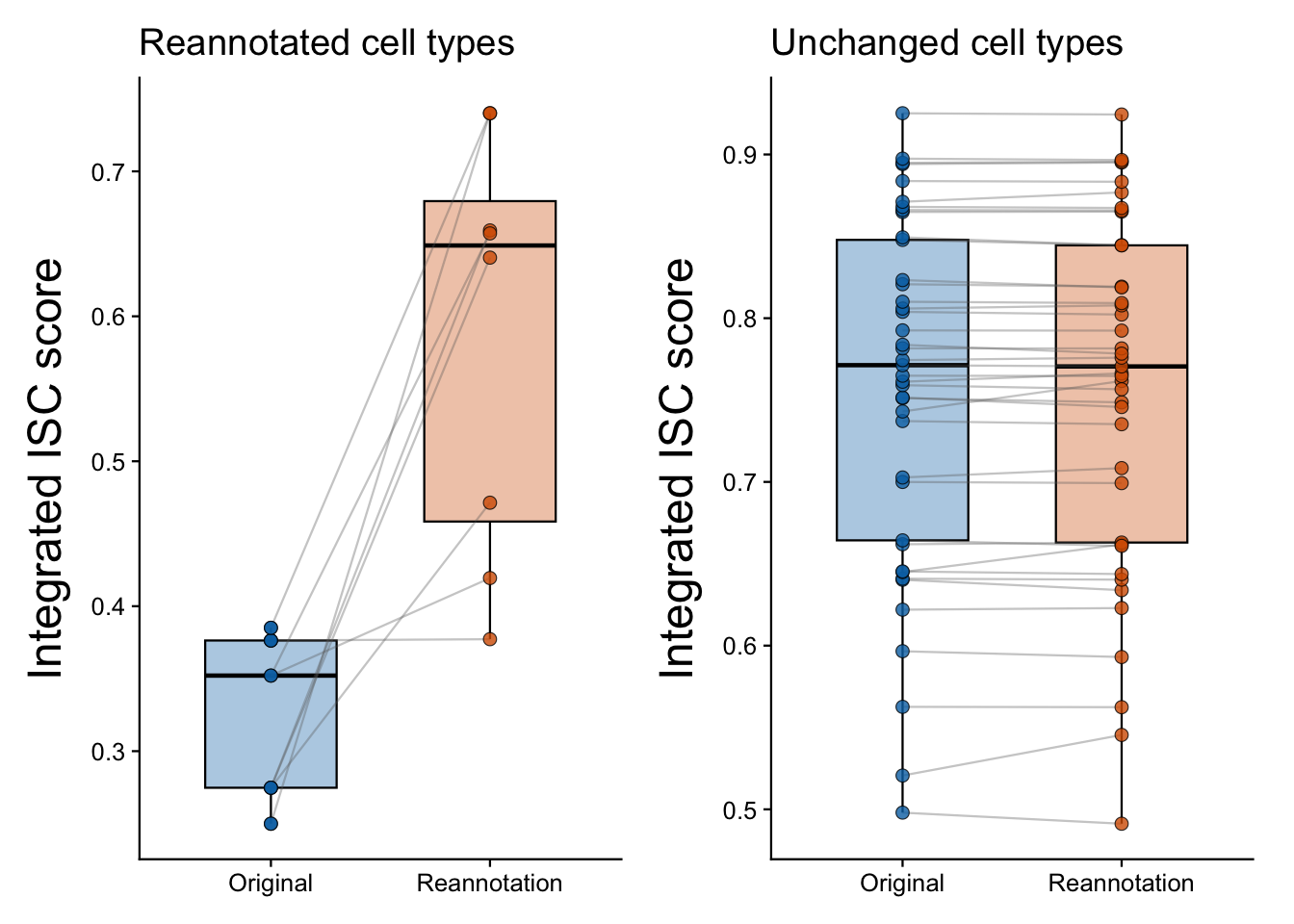
We define the integrated score as the product of local and global ISC per cell type. Let’s explore how much this integrated score improved after the annotation changes we applied.

First, harmonize and unify consistency scores before (original) and after reannotation (refined).

dfp <- rbind(cons_original %>% mutate(ident = "original"),
             cons_refined %>%
               mutate(ident = "reannot"
                      )) %>% 
  select(celltype, score = integrated_isc, ident)
dict <- metadata_refined %>% 
  mutate(cell_type = scTypeEval:::purge_label(cell_type),
         annot2 = scTypeEval:::purge_label(annot2)
  ) %>% 
  distinct(cell_type, annot2) %>% 
  dplyr::rename("celltype" = "annot2")

spl <- split(dfp, dfp$ident)

spl$reannot <- left_join(spl$reannot, dict, by = "celltype") %>% 
  rename("newannot" = "celltype",
         "celltype" = "cell_type",
         "score2" = "score")

dfp2 <- left_join(spl$original, spl$reannot,
                  by = "celltype") %>% 
  mutate(
    scoref = score2 - score,
    #scoref = log2(score2/score),
    is.newannot = ifelse(celltype == newannot,
                         "no", "yes")
  )
dfp2 <- dfp2[,!grepl("ident", names(dfp2))]

dd <- dfp2 %>% 
  select(-scoref) %>% 
  dplyr::rename("Reannotation" = "score2",
                "Original" = "score") %>% 
  pivot_longer(-c(celltype, newannot, is.newannot),
               names_to = "annotation",
               values_to = "score")

Plot ISC changes for unmodified and modified annotation labels

nm_cols <- c(
  "#0072B2",
  "#D55E00"
)
limits <- c(min(dd$score) * 0.9,
            max(dd$score) * 1.05)
titles_dict <- c("yes" = "Reannotated cell types",
                 "no" = "Unchanged cell types")
pl3 <- lapply(c("yes", "no"), function(i) {
  title <- titles_dict[i]
  dd_sub <- dd %>%
    filter(is.newannot == i) %>%
    mutate(g = paste(celltype, newannot, sep = "__"))
  ggplot(dd_sub, aes(annotation, score, fill = annotation)) +
    # Boxplot
    geom_boxplot(
      width = 0.6,
      outlier.shape = NA,
      alpha = 0.35,
      color = "black",
      linewidth = 0.4
    ) +
    # Connecting lines
    geom_line(
      aes(group = g),
      color = "grey40",
      alpha = 0.35,
      linewidth = 0.4
    ) +
    # Points
    geom_point(
      shape = 21,
      size = 2.2,
      stroke = 0.3,
      alpha = 0.8,
      color = "black"
    ) +
    scale_fill_manual(values = nm_cols) +
    coord_cartesian(ylim = limits) +
    labs(
      y = "Integrated ISC score",
      x = NULL,
      title = title
    ) +
    theme_classic(base_size = 12) +
    theme(
      legend.position = "none",
      axis.title.y = element_text(margin = margin(r = 8),
                                  size = 18),
      axis.line = element_line(linewidth = 0.4),
      axis.ticks = element_line(linewidth = 0.4),
      plot.margin = margin(5, 10, 5, 5)
    )
})

patchwork::wrap_plots(pl3)

11.2 Movement in local/global ISC space

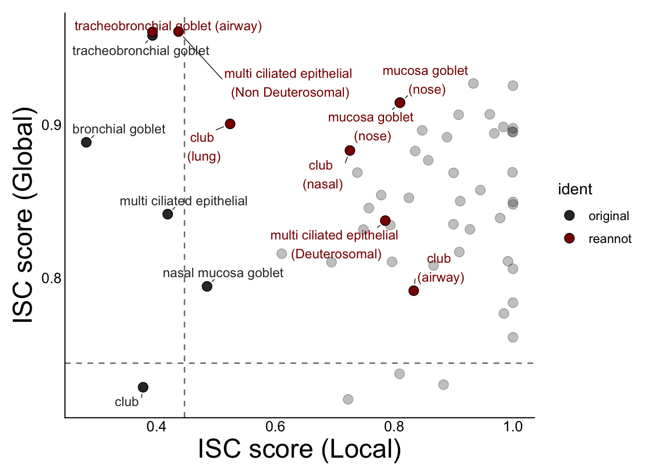
Let’s visualize how the reannotations applied change the position of the labels in the ISC local-global space.

# function to make label aesthetics
clean_ident_labels <- function(x) {
  x |>
    gsub("\\.\\(", "\n(", x = _) |>   # ".(" -> newline
    gsub("\\.", " ", x = _) |>        # "." -> space
    gsub("\\bcell\\b", "", x = _) |>  # remove standalone "cell"
    gsub(" +", " ", x = _) |>         # collapse multiple spaces
    trimws()
}

dfp <- rbind(cons_original %>% mutate(ident = "original"),
             cons_refined %>%
               mutate(ident = "reannot")
             ) 
dict <- metadata_refined %>% 
  mutate(cell_type = scTypeEval:::purge_label(cell_type),
         annot2 = scTypeEval:::purge_label(annot2)
  ) %>% 
  distinct(cell_type, annot2) %>% 
  dplyr::rename("celltype" = "annot2")

dfp2 <- left_join(dfp, dict, by = "celltype") %>% 
  mutate(pair_id = coalesce(cell_type, celltype)) %>%
  filter(!(ident == "reannot" & celltype == cell_type)) %>% 
  mutate(highlight = ifelse(is.na(cell_type) | ident == "reannot",
         "yes", "no"),
         celltype = clean_ident_labels(celltype),
         cell_type = clean_ident_labels(cell_type)
         )
cols <- c("original"  = "grey20", "reannot" = "red4")
vals <- c("yes" = 1, "no" = 0.3)
imp_scatter <- dfp2 %>%
  ggplot(aes(x = local,
             y = global,
             alpha = highlight)) +
  geom_vline(
    xintercept = q_local,
    linetype = "dashed",
    linewidth = 0.5,
    alpha = 0.6
  ) +
  geom_hline(
    yintercept = q_global,
    linetype = "dashed",
    linewidth = 0.5,
    alpha = 0.6
  ) +
  # Points
  geom_point(aes(fill = ident),
             shape = 21,
             size = 3.2,
             stroke = 0.4,
             color = "black",
             show.legend = T) +
  scale_fill_manual(values = cols) +
  # Repelled labels (better spacing control)
  ggrepel::geom_text_repel(
    aes(label = ifelse(highlight == "yes",
                       celltype, NA),
        color = ident),
    size = 3.5,
    max.overlaps = 20,
    box.padding = 0.4,
    point.padding = 0.3,
    segment.size = 0.3,
    segment.color = "grey15",
    min.segment.length = 0,
    seed = 123,
    show.legend = F
  ) +
  scale_color_manual(values = cols) +
  scale_alpha_manual(values = vals) +
  guides(alpha = "none") +
  
  labs(
    x = "ISC score (Local)",
    y = "ISC score (Global)"
  ) +
  
  coord_cartesian(clip = "off") +
  
  theme_classic(base_size = 12) +
  theme(
    axis.title = element_text(size = 20),
    axis.text  = element_text(size = 11),
    axis.line  = element_line(linewidth = 0.4),
    axis.ticks = element_blank(),
    plot.margin = margin(10, 20, 10, 10)
  )
imp_scatter

We can see from both the boxplot and the ISC scatter plot that the proposed reannotation successfully increases the ISC of the modified epithelial populations while leaving the remaining cell type labels largely unchanged. In particular, club cells, initially characterized by low ISCL and ISCG, showed concurrent increases in both metrics upon splitting into tissue-resolved subtypes, reflecting recovery of both inter-sample compactness and replicability. Likewise, merging bronchial and nasal goblet cells into a common mucosa goblet cell label improves local consistency, suggesting that these annotations were previously over-partitioned. Together, these results illustrate how ISC can be used not only to identify annotations that warrant refinement, but also to quantitatively validate that targeted changes improve annotation consistency without perturbing well-defined cell types.

12 Interpretation

This case study shows that low ISC in HLCA epithelial annotations is not simply technical noise, but largely reflects biologically structured heterogeneity linked to tissue context. By using ISC diagnostics to target specific low-consistency labels and refining them with metadata-informed splits (and selective merges), the revised annotation framework increases consistency where expected while preserving stable annotations elsewhere. Overall, the workflow demonstrates a practical strategy to move from a broad consensus atlas annotation toward a more reproducible and biologically interpretable labeling scheme across individuals.
13 Session information

sessionInfo()
R version 4.6.0 alpha (2026-03-31 r89754)
Platform: aarch64-apple-darwin23
Running under: macOS Tahoe 26.5.1

Matrix products: default
BLAS:   /Library/Frameworks/R.framework/Versions/4.6/Resources/lib/libRblas.0.dylib 
LAPACK: /Library/Frameworks/R.framework/Versions/4.6/Resources/lib/libRlapack.dylib;  LAPACK version 3.12.1

locale:
[1] en_US.UTF-8/en_US.UTF-8/en_US.UTF-8/C/en_US.UTF-8/en_US.UTF-8

time zone: Europe/Zurich
tzcode source: internal

attached base packages:
[1] stats     graphics  grDevices datasets  utils     methods   base     

other attached packages:
[1] Seurat_5.5.1       SeuratObject_5.4.0 sp_2.2-1           scTypeEval_1.0.0  
[5] ggplot2_4.0.3      tidyr_1.3.2        dplyr_1.2.1       

loaded via a namespace (and not attached):
  [1] RColorBrewer_1.1-3          rstudioapi_0.19.0          
  [3] jsonlite_2.0.0              magrittr_2.0.5             
  [5] spatstat.utils_3.2-3        farver_2.1.2               
  [7] rmarkdown_2.31              vctrs_0.7.3                
  [9] ROCR_1.0-12                 spatstat.explore_3.8-1     
 [11] htmltools_0.5.9             S4Arrays_1.12.0            
 [13] BiocNeighbors_2.6.0         SparseArray_1.12.2         
 [15] sctransform_0.4.3           parallelly_1.48.0          
 [17] KernSmooth_2.23-26          htmlwidgets_1.6.4          
 [19] ica_1.0-3                   plyr_1.8.9                 
 [21] plotly_4.12.0               zoo_1.8-15                 
 [23] igraph_2.3.3                mime_0.13                  
 [25] lifecycle_1.0.5             pkgconfig_2.0.3            
 [27] rsvd_1.0.5                  Matrix_1.7-5               
 [29] R6_2.6.1                    fastmap_1.2.0              
 [31] MatrixGenerics_1.24.0       fitdistrplus_1.2-6         
 [33] future_1.70.0               shiny_1.14.0               
 [35] digest_0.6.39               patchwork_1.3.2            
 [37] S4Vectors_0.50.1            tensor_1.5.1               
 [39] dqrng_0.4.1                 RSpectra_0.16-2            
 [41] irlba_2.3.7                 GenomicRanges_1.64.0       
 [43] beachmat_2.28.0             labeling_0.4.3             
 [45] progressr_1.0.0             spatstat.sparse_3.2-0      
 [47] httr_1.4.8                  polyclip_1.10-7            
 [49] abind_1.4-8                 compiler_4.6.0             
 [51] withr_3.0.3                 S7_0.2.2                   
 [53] BiocParallel_1.46.0         fastDummies_1.7.6          
 [55] MASS_7.3-65                 DelayedArray_0.38.2        
 [57] bluster_1.22.0              tools_4.6.0                
 [59] lmtest_0.9-40               otel_0.2.0                 
 [61] httpuv_1.6.17               future.apply_1.20.2        
 [63] goftest_1.2-3               glue_1.8.1                 
 [65] nlme_3.1-169                promises_1.5.0             
 [67] grid_4.6.0                  Rtsne_0.17                 
 [69] cluster_2.1.8.2             reshape2_1.4.5             
 [71] generics_0.1.4              gtable_0.3.6               
 [73] spatstat.data_3.1-9         data.table_1.18.4          
 [75] utf8_1.2.6                  metapod_1.20.0             
 [77] ScaledMatrix_1.20.0         BiocSingular_1.28.0        
 [79] XVector_0.52.0              BiocGenerics_0.58.1        
 [81] spatstat.geom_3.8-1         RcppAnnoy_0.0.23           
 [83] ggrepel_0.9.8               RANN_2.6.2                 
 [85] pillar_1.11.1               stringr_1.6.0              
 [87] limma_3.68.4                spam_2.11-4                
 [89] RcppHNSW_0.7.0              later_1.4.8                
 [91] splines_4.6.0               lattice_0.22-9             
 [93] renv_1.2.3                  survival_3.8-6             
 [95] deldir_2.0-4                tidyselect_1.2.1           
 [97] locfit_1.5-9.12             SingleCellExperiment_1.34.0
 [99] scuttle_1.22.0              miniUI_0.1.2               
[101] pbapply_1.7-4               knitr_1.51                 
[103] gridExtra_2.3.1             IRanges_2.46.0             
[105] Seqinfo_1.2.0               edgeR_4.10.1               
[107] SummarizedExperiment_1.42.0 scattermore_1.2            
[109] stats4_4.6.0                xfun_0.60                  
[111] Biobase_2.72.0              statmod_1.5.2              
[113] matrixStats_1.5.0           stringi_1.8.7              
[115] lazyeval_0.2.3              yaml_2.3.12                
[117] evaluate_1.0.5              codetools_0.2-20           
[119] tibble_3.3.1                cli_3.6.6                  
[121] uwot_0.2.4                  xtable_1.8-8               
[123] reticulate_1.46.0           Rcpp_1.1.2                 
[125] globals_0.19.1              spatstat.random_3.5-0      
[127] png_0.1-9                   spatstat.univar_3.2-0      
[129] parallel_4.6.0              dotCall64_1.2              
[131] scran_1.40.0                listenv_1.0.0              
[133] viridisLite_0.4.3           scales_1.4.0               
[135] ggridges_0.5.7              purrr_1.2.2                
[137] rlang_1.3.0                 cowplot_1.2.0