White adipose tissue atlas

Authors
Affiliation

Josep Garnica

University of Geneva

Sophie Barakat

University of Geneva

Published

July 16, 2026

1 Introduction

In this case study, we evaluate the consistency of the cell type annotations provided by the authors of a white adipose tissue atlas.

2 Dataset description

Emont et al., 2022 generated a single-cell atlas of human and mouse white adipose tissue across multiple depots, donors, and adipose cell compartments. The atlas captures the major adipose, stromal/vascular, and immune populations, including adipocytes, adipocyte progenitors, endothelial cells, fibroblasts/pericytes, and resident leukocytes. For this case study, we use the human white adipose tissue object distributed through SCP1376, which contains 166,149 cells and the accompanying metadata used for downstream annotation consistency analyses.

3 Download data

Data can be found at SCP1376. We will download lite objects that only contain RNA data and thus are easier to download.

url <- paste0(
  "https://uchicago.box.com/s/bmhkw0j2qkkgnpmpz33bw583pppoib0y"
)
cache_dir <- file.path("cache")
dir.create(cache_dir, recursive = TRUE, showWarnings = FALSE)
dataset_file <- file.path(
  cache_dir,
  "human_all_lite.rds"
)
if (!file.exists(dataset_file)) {
  # increase timeout, file size is 1.3 GB
  old_timeout <- getOption("timeout")
  on.exit(options(timeout = old_timeout), add = TRUE)
  options(timeout = 99999)
  utils::download.file(url, dataset_file, mode = "wb")
}
dataset_file
[1] "cache/human_all_lite.rds"

4 Load packages and constants

library(dplyr)
library(tidyr)
library(ggplot2)
library(scTypeEval)
library(Seurat)
theme_set(theme_bw(base_size = 12))
# Blacklisted genes that are inherently variable across samples
# and should be excluded from ISC (scTypeEval) computations
data(black_list)
blacklist_genes <- c(black_list$TCR, black_list$Immunoglobulins, black_list$Ygenes)
# These are the local and global ISC thresholds empirically described in the manuscript (Fig. 5)
q_local <- 0.4467538
q_global <- 0.7443436

5 Load Human WAT atlas dataset

# this function load Seurat, SCE, or AnnData object and returns
# a list with 1) counts and 2) metadata if `split = TRUE`
hwat <- load_single_cell_object(dataset_file,
                                split = T)
# split into metadata and counts
metadata <- hwat$metadata
counts <- hwat$counts
dim(counts)
[1]  31533 166149

Dataset consists of >166k cells.

5.1 Explore metadata

For the scTypeEval pipeline we need to identify: 1. the individual of origin: individual (22 patients in total) 2. the author’s annotation or clustering, or another cell classification derived from gene expression: - cell_type2: Broad annotation - cell_type: Fine annotation

Explore sample-level metadata

# Define important patient/sample-wise variables
patient_vars <- c("sample", "individual",
                  "race", "source", "depot",
                  "tissue",
                  "age", "bmi" )
sample_lev_metadata <- metadata %>% 
  distinct(sample, .keep_all = T) %>% 
  select(all_of(patient_vars)) %>% 
  tibble::remove_rownames()
sample_lev_metadata
           sample individual      race        source depot  tissue age   bmi
1       Hs_OAT_12      Hs012 Caucasian       Omental   VAT adipose nan 48.80
2       Hs_SAT_12      Hs012 Caucasian Periumbilical   SAT adipose nan 48.80
3       Hs_OAT_13      Hs013 Caucasian       Omental   VAT adipose nan 43.20
4       Hs_SAT_13      Hs013 Caucasian Periumbilical   SAT adipose nan 43.20
5      Hs_OAT_266      Hs266 Caucasian       Omental   VAT adipose  68 22.15
6      Hs_SAT_266      Hs266 Caucasian Periumbilical   SAT adipose  68 22.15
7       Hs_OAT_01      Hs001 Caucasian       Omental   VAT adipose  29 42.70
8       Hs_SAT_01      Hs001 Caucasian Periumbilical   SAT adipose  29 42.70
9       Hs_SAT_02      Hs002 Caucasian Periumbilical   SAT adipose  57 33.20
10      Hs_SAT_04      Hs004 Caucasian Periumbilical   SAT adipose  51 25.30
11     Hs_OAT_253      Hs253 Caucasian Preperitoneal   VAT adipose  53 30.04
12     Hs_SAT_253      Hs253 Caucasian Periumbilical   SAT adipose  53 30.04
13     Hs_OAT_254      Hs254 Caucasian Preperitoneal   VAT adipose  41 23.96
14     Hs_SAT_254      Hs254 Caucasian Periumbilical   SAT adipose  41 23.96
15     Hs_OAT_256      Hs256     Black       Omental   VAT adipose  41 34.53
16     Hs_SAT_256      Hs256     Black Periumbilical   SAT adipose  41 34.53
17     Hs_OAT_255      Hs255 Caucasian Preperitoneal   VAT adipose  73 24.27
18     Hs_SAT_255      Hs255 Caucasian Periumbilical   SAT adipose  73 24.27
19      Hs_OAT_09      Hs009 Caucasian       Omental   VAT adipose  41 45.70
20      Hs_SAT_09      Hs009 Caucasian Periumbilical   SAT adipose  41 45.70
21      Hs_OAT_10      Hs010 Caucasian       Omental   VAT adipose  35 43.10
22      Hs_SAT_10      Hs010 Caucasian Periumbilical   SAT adipose  35 43.10
23      Hs_SAT_11      Hs011     Black Periumbilical   SAT adipose  58 42.80
24 Hs_SAT_SVF_235      Hs235 Caucasian        Pannus   SAT     SVF  53 36.00
25 Hs_SAT_SVF_236      Hs236 Caucasian         Thigh   SAT     SVF  35 26.00
26 Hs_SAT_SVF_237      Hs237 Caucasian        Pannus   SAT     SVF  53 23.00
27 Hs_SAT_SVF_238      Hs238 Caucasian        Pannus   SAT     SVF  49 20.00
28 Hs_SAT_SVF_239      Hs239 Caucasian        Pannus   SAT     SVF  71 25.00
29 Hs_SAT_SVF_240      Hs240 Caucasian        Pannus   SAT     SVF  59 26.00
30 Hs_SAT_SVF_242      Hs242 Caucasian        Pannus   SAT     SVF  59 23.00
31 Hs_SAT_SVF_248      Hs248 Caucasian        Pannus   SAT     SVF  68 32.00
32 Hs_SAT_SVF_249      Hs249 Caucasian        Pannus   SAT     SVF  54 26.00

5.1.1 Explore annotations and metadata

We follow the standard Seurat processing workflow to explore UMAPs for this dataset. We first define a helper function for these steps.

processing_seurat <- function(seu,
                              nfeatures = 2000,
                              npcs = 30,
                              umaps_dim = 30,
                              verbose = F){
  seu <- NormalizeData(seu, verbose = FALSE)
  seu <- FindVariableFeatures(
    seu,
    selection.method = "vst",
    nfeatures = nfeatures,
    verbose = FALSE
  )
  seu <- ScaleData(
    seu,
    verbose = FALSE
  )
  seu <- RunPCA(
    seu,
    npcs = npcs,
    verbose = verbose
  ) 
  # Compute UMAP
  seu <- RunUMAP(
    seu,
    dims = 1:umaps_dim,
    verbose = verbose
  ) 
  return(seu)
} 
# Create seurat object
seu <- CreateSeuratObject(
  counts = counts,
  meta.data = metadata
)
seu <- processing_seurat(seu)

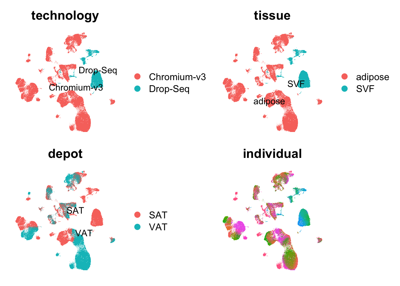
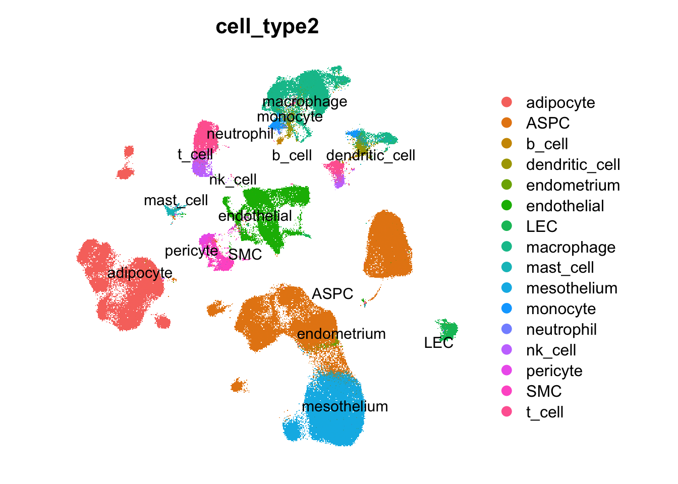
Visually explore the different metadata information by looking at the UMAPs.

vars <- c("technology",
          "tissue",
          "depot",
          "individual",
          "cell_type2"
)
umap_expl <- lapply(vars, function(v){
  lab <- ifelse(n_distinct(seu@meta.data[[v]]) < 20,
                T, F)
  pl <- DimPlot(
    seu,
    group.by = v,
    label = lab,
    repel = TRUE,
    raster = TRUE
  ) + 
    NoAxes() +
    theme(aspect.ratio = 1)
  # do not show legend if too many values
  if(!lab){
    pl <- pl + NoLegend()
  }
  return(pl)
})  

patchwork::wrap_plots(umap_expl[1:4],
                      ncol = 2)

umap_expl[[5]]

5.2 Dataset filtering

Because tissue of origin, depot, and technology are not balanced, we keep only Chromium-v3, the most abundant technology in the dataset. This protocol uses single-nucleus RNA-seq (snRNA-seq), which, unlike whole-cell approaches, captures adipocytes and mesothelial cells more effectively. The authors also used these snRNA-seq data to build the atlas. See the original paper for more details.

seu_chromv3 <- seu[,seu$technology == "Chromium-v3"]
dim(seu_chromv3)
[1]  31533 137684

6 Inter-Sample Consistency (ISC) metrics on Broad annotation

We will start by evaluating the ISC of broad annotation provided by authors (metadata column cell_type2)

For that we will perform the full ISC analysis pipeline: 1.Create a scTypeEval object from counts and metadata. 2.Process the data and define samples/cell type annotations. 3.Select highly variable genes (HVGs). 4.Compute a PCA embedding. 5.Calculate local and global dissimilarities. 6.Compute consistency metrics. 7.Build the final Integrated ISC table.

6.1 Process data and obtain Highly Variable Genes

ident <- "cell_type2" # broad annotation
# use filtered Seurat object with only Chromimum v3 snNuc-seq
sceval <- create_scTypeEval(seu_chromv3) 

sceval_broad <- run_processing_data(
  scTypeEval = sceval,
  ident = ident, # in this case broad annotation
  sample = "individual",
  min_samples = 5,
  min_cells = 10,
  verbose = FALSE
)
sceval_broad <- run_hvg(
  scTypeEval = sceval_broad,
  ngenes = 2000,
  sample = TRUE,
  aggregation = "single-cell",
  black_list = blacklist_genes,
  ncores = 4,
  verbose = FALSE
)

6.2 Add embedding (run_pca)

# remove data from single-cell grouping as we don't need it
# to compute ISC other than WasserStein
sceval_broad@data$`single-cell` <- NULL
set.seed(22)
sceval_broad <- run_pca(
  scTypeEval = sceval_broad,
  ndim = 30,
  verbose = FALSE
)
# Visualize PCA by cell type and samples groups
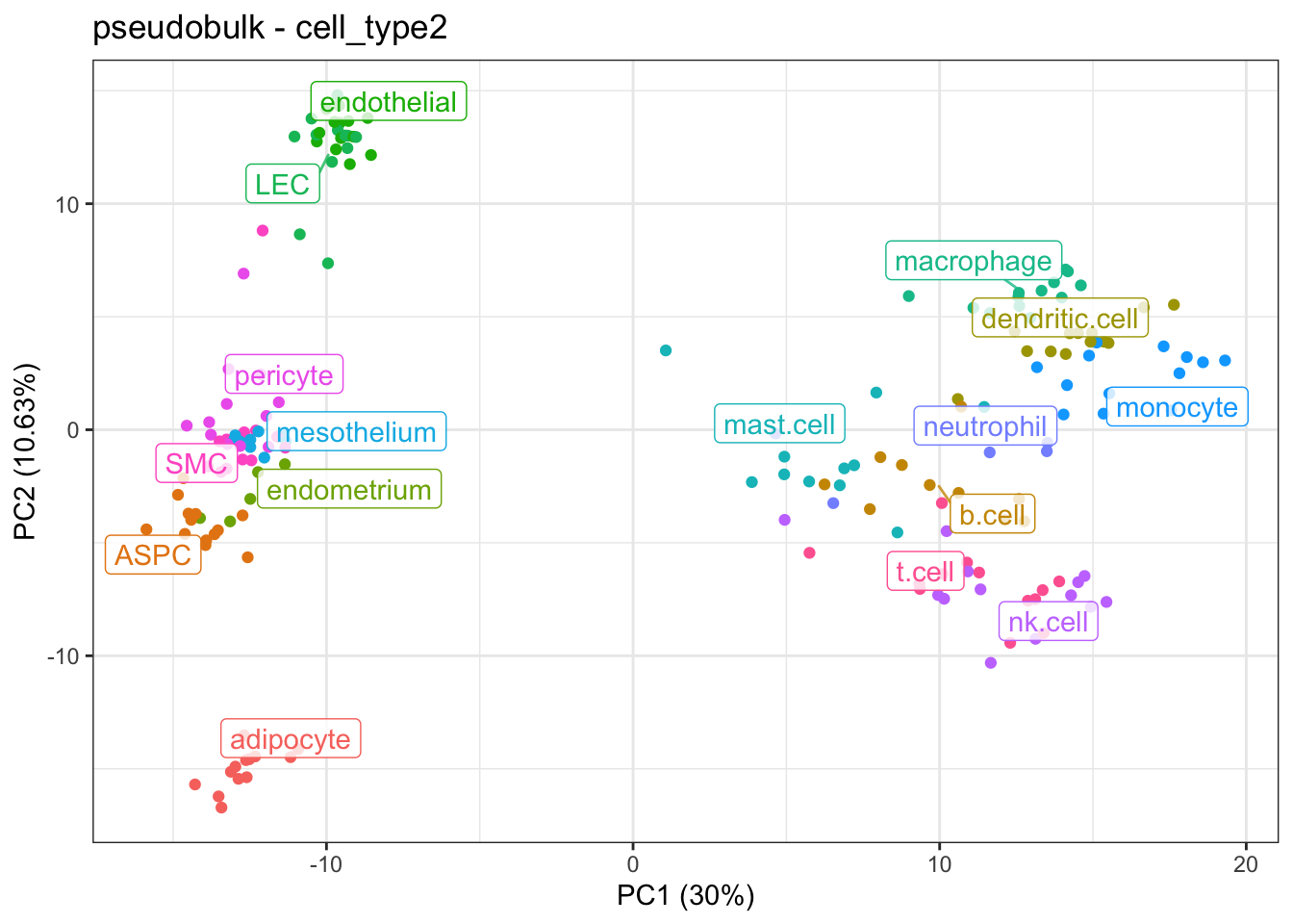
plot_pca(sceval_broad)

We can observe the individual-wise cell type variability, clearly separating the immune and non-immune compartment

6.3 Compute dissimilarities (run_dissimilarity)

Build pairwise distance matrices between all cell types & sample pairs

sceval_broad <- run_dissimilarity(
  sceval_broad,
  method = "recip_classif:Match",
  reduction = FALSE,
  ncores = 4,
  verbose = FALSE
)
sceval_broad <- run_dissimilarity(
  sceval_broad,
  method = "Pseudobulk:Cosine",
  reduction = TRUE,
  verbose = FALSE
)
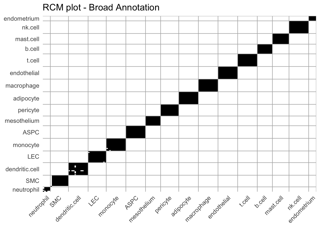
# Visualize reciprocal classification match (RCM) plot
# This inform us of the cross-sample reproducbility of each annotation
plot_heatmap(sceval_broad,
            dissimilarity_slot = "recip_classif:Match", 
            sort_consistency = "silhouette",
            sort_similarity = "Pseudobulk:Cosine")+
  ggtitle("RCM plot - Broad Annotation")

RCM plot is already telling us that authors broad annotation (cell_type2) is highly reproducible across samples, showing clear on-diagonal blocks.

6.4 Compute consistency (get_consistency)

We then compute the consistency metrics from the previously generated distance matrices. We use global and local ISC, defined here as 2-label silhouette + pseudobulk cosine and silhouette + recip_classif:Match, respectively. For additional details, see Benchmarking of ISC metrics.

cons_broad_raw <- get_consistency(
  sceval_broad,
  dissimilarity_slot = c("recip_classif:Match", "Pseudobulk:Cosine"),
  consistency_metric = c("silhouette", "2label_silhouette")
)

### Build local/global ISC table
cons_broad <- cons_broad_raw |>
  mutate(method.type = paste(consistency_metric, dissimilarity_method, sep = " | ")) |>
  filter(method.type %in% c(
    "silhouette | recip_classif:Match",
    "2label_silhouette | Pseudobulk:Cosine"
  )) |>
  mutate(
    metric = factor(
      method.type,
      levels = c(
        "silhouette | recip_classif:Match",
        "2label_silhouette | Pseudobulk:Cosine"
      ),
      labels = c("local", "global")
    )
  ) |>
  select(celltype, metric, measure) |>
  pivot_wider(names_from = metric, values_from = measure) |>
  mutate(integrated_isc = local * global) |>
  arrange(integrated_isc)

The final object (cons_broad) contains, for each cell type: - Local ISC: silhouette + recip_classif:Match - Global ISC: 2-label silhouette + pseudobulk cosine - Integrated ISC (local × global)

Show scatter of global and local ISC

cons_broad %>%
  ggplot(aes(x = local,
             y = global)) +
  # threshold line of figure 5
  geom_vline(
    xintercept = q_local,
    linetype = "dashed",
    linewidth = 0.5,
    alpha = 0.6
  ) +
  geom_hline(
    yintercept = q_global,
    linetype = "dashed",
    linewidth = 0.5,
    alpha = 0.6
  ) +
  # Points
  geom_point(aes(fill = integrated_isc),
             shape = 21,
             size = 3.2,
             stroke = 0.4,
             color = "black",
             alpha = 0.9,
             show.legend = FALSE) +
  
  # Clean blue gradient (Nature-friendly, perceptually smooth)
  scale_fill_gradient(
    low  = "#F7FBFF",
    high = "#08306B"
  ) +
  
  # Repelled labels (better spacing control)
  ggrepel::geom_text_repel(
    aes(label = celltype),
    size = 3.5,
    max.overlaps = 8,
    box.padding = 0.4,
    point.padding = 0.3,
    segment.size = 0.3,
    segment.color = "grey50",
    min.segment.length = 0,
    seed = 22
  ) +
  labs(
    x = "ISCL (silhouette on recip_classif:Match)",
    y = "ISCG (2label_silhouette on Pseudobulk:Cosine)",
    title = "WAT Atlas broad cell types in ISC space"
  ) +
  coord_cartesian(clip = "off") +
  theme_classic(base_size = 12)

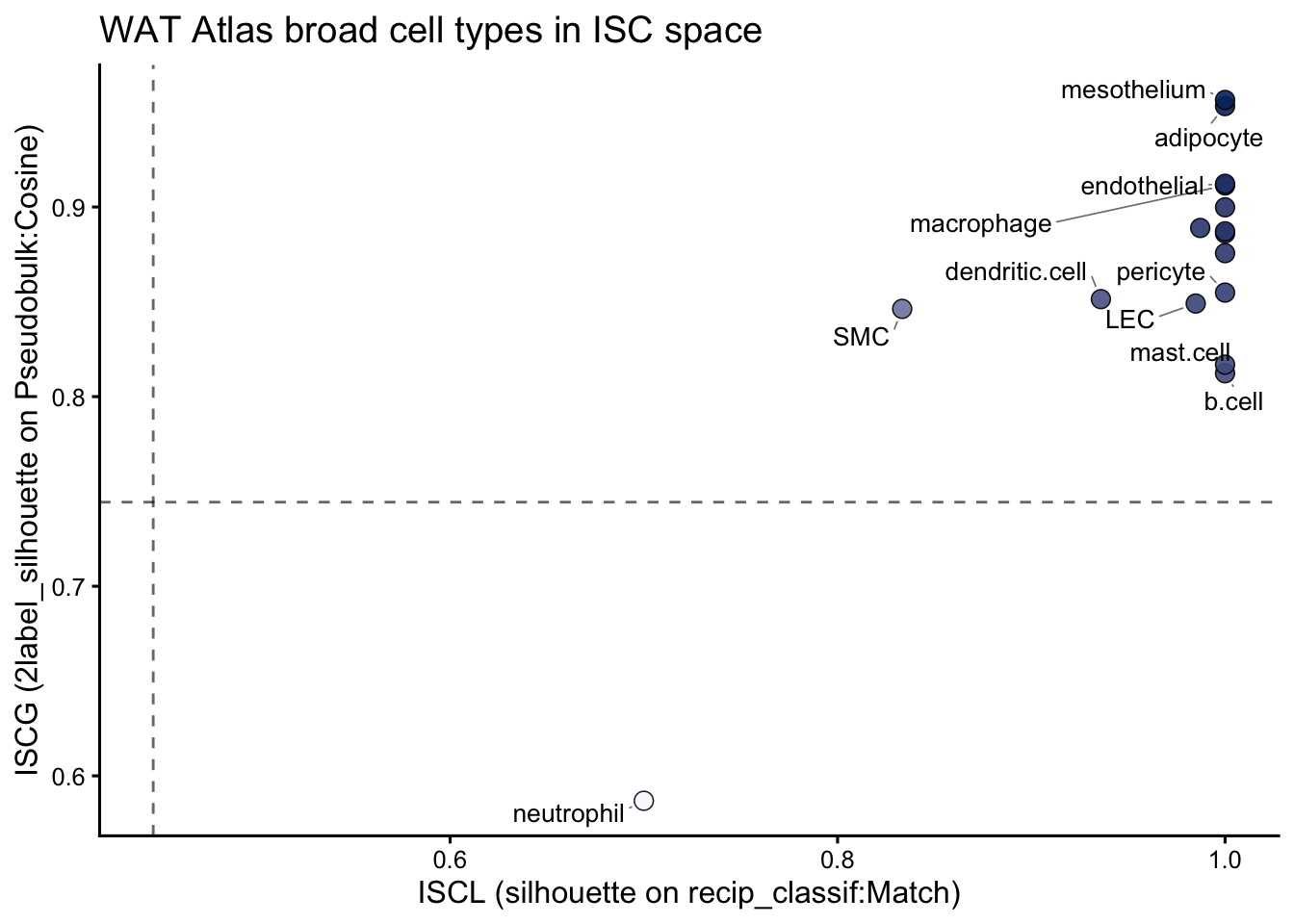
All broad annotation labels, except neutrophils, are above the empirical thresholds reported for these metrics, suggesting that this annotation framework is highly reproducible. Neutrophils are usually reported to have lower quality in single-cell RNA-seq datasets due to their intrinsic fragility during tissue dissociation and sample processing. Their sensitivity to handling conditions can lead to increased RNA degradation, reduced transcript complexity, and greater technical variability, which may negatively impact consistency-based evaluation metrics. Some immune cell types, including dendritic cells, mast cells, B cells, and NK cells, show global ISC below 0.9, which suggests some room for improvement through finer subdivision.

7 Inter-Sample Consistency (ISC) metrics on fine annotation

We next repeat the same pipeline for the authors’ finer annotation (cell_type).

7.1 Process data and obtain Highly Variable Genes

ident <- "cell_type" # author's fine annotation
sceval_fine <- run_processing_data(
  scTypeEval = sceval,
  ident = ident, # in this case broad annotation
  sample = "individual",
  min_samples = 5,
  min_cells = 10,
  verbose = FALSE
)
sceval_fine <- run_hvg(
  scTypeEval = sceval_fine,
  ngenes = 2000,
  sample = TRUE,
  aggregation = "single-cell",
  black_list = blacklist_genes,
  ncores = 4,
  verbose = FALSE
)

7.2 Add embedding (run_pca)

# remove data from single-cell grouping as we don't need it
sceval_fine@data$`single-cell` <- NULL
sceval_fine <- run_pca(
  scTypeEval = sceval_fine,
  ndim = 30,
  verbose = FALSE
)
# Visualize PCA by cell type and samples groups
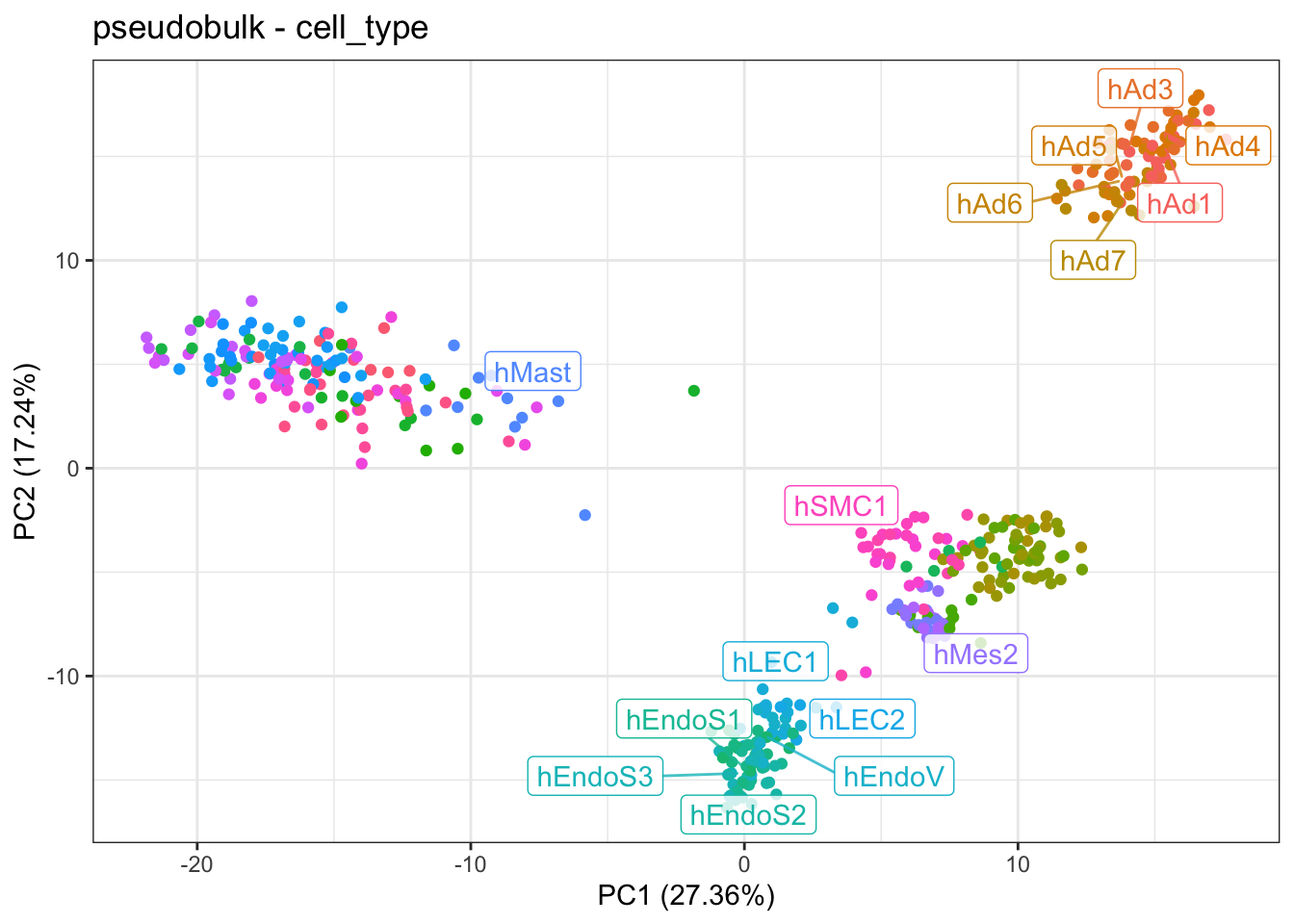
plot_pca(sceval_fine)

7.3 Compute dissimilarities (run_dissimilarity)

sceval_fine <- run_dissimilarity(
  sceval_fine,
  method = "recip_classif:Match",
  reduction = FALSE,
  ncores = 4,
  verbose = FALSE
)
sceval_fine <- run_dissimilarity(
  sceval_fine,
  method = "Pseudobulk:Cosine",
  reduction = TRUE,
  verbose = FALSE
)
# Visualize reciprocal classification match (RCM) plot
plot_heatmap(sceval_fine,
            dissimilarity_slot = "recip_classif:Match", 
            sort_consistency = "silhouette",
            sort_similarity = "Pseudobulk:Cosine") +
  ggtitle("RCM plot - Fine annotation")

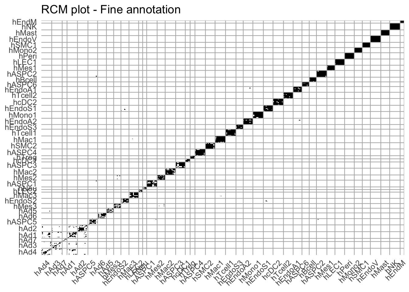
Based on the RCM plot, some cell types show high reproducibility across samples (for example, SMC1, Peri, Tcell1, and Mac1), whereas others, particularly adipocyte subtypes, show a much lower rate of reproducibility. This suggests that some of these adipocyte subtypes are more similar to other subtypes from the same sample than to the same subtype across samples.

7.4 Compute consistency (get_consistency)

cons_fine_raw <- get_consistency(
  sceval_fine,
  dissimilarity_slot = c("recip_classif:Match", "Pseudobulk:Cosine"),
  consistency_metric = c("silhouette", "2label_silhouette")
)
### Build local/global ISC table
cons_fine <- cons_fine_raw |>
  mutate(method.type = paste(consistency_metric, dissimilarity_method, sep = " | ")) |>
  filter(method.type %in% c(
    "silhouette | recip_classif:Match",
    "2label_silhouette | Pseudobulk:Cosine"
  )) |>
  mutate(
    metric = factor(
      method.type,
      levels = c(
        "silhouette | recip_classif:Match",
        "2label_silhouette | Pseudobulk:Cosine"
      ),
      labels = c("local", "global")
    )
  ) |>
  select(celltype, metric, measure) |>
  pivot_wider(names_from = metric, values_from = measure) |>
  mutate(integrated_isc = local * global) |>
  arrange(integrated_isc)

Show scatter of global and local ISC

cons_fine %>%
  ggplot(aes(x = local,
             y = global)) +
  # threshold line of figure 5
  geom_vline(
    xintercept = q_local,
    linetype = "dashed",
    linewidth = 0.5,
    alpha = 0.6
  ) +
  geom_hline(
    yintercept = q_global,
    linetype = "dashed",
    linewidth = 0.5,
    alpha = 0.6
  ) +
  # Points
  geom_point(aes(fill = integrated_isc),
             shape = 21,
             size = 3.2,
             stroke = 0.4,
             color = "black",
             alpha = 0.9,
             show.legend = FALSE) +
  
  # Clean blue gradient (Nature-friendly, perceptually smooth)
  scale_fill_gradient(
    low  = "#F7FBFF",
    high = "#08306B"
  ) +
  
  # Repelled labels (better spacing control)
  ggrepel::geom_text_repel(
    aes(label = celltype),
    size = 3.5,
    max.overlaps = 8,
    box.padding = 0.4,
    point.padding = 0.3,
    segment.size = 0.3,
    segment.color = "grey50",
    min.segment.length = 0,
    seed = 22
  ) +
  
  labs(
    x = "ISCL (silhouette on recip_classif:Match)",
    y = "ISCG (2label_silhouette on Pseudobulk:Cosine)",
    title = "WAT Atlas fine cell types in ISC space"
  ) +
  coord_cartesian(clip = "off") +
  theme_classic(base_size = 12)

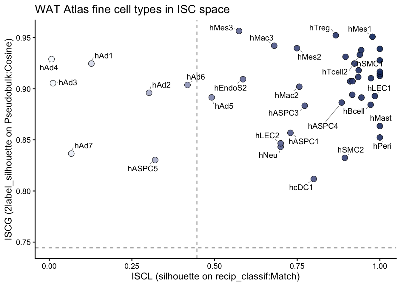
The local versus global ISC scatter plot confirms the pattern suggested by the RCM plot. Most adipocyte subtypes (hAd*) fall below the empirical threshold for local consistency, suggesting that these labels reflect over-partitioning of adipocyte populations that are not reproducibly separated across samples.

This interpretation is also consistent with the paper, where the molecular distinction between adipocyte subpopulations appears limited based on the reported marker specificity, as shown in Fig. 3A and Extended Data Fig. 9:

Characterization of human adipocyte subtypes. Source: Emont et al., 2022. Extended Data Fig. 9

8 Reannotation of adipocytes

After finding that the adipocyte subtypes in the authors’ fine annotation do not show good cross-sample reproducibility, we can test alternative annotations guided by this criterion. We therefore explore sample-level metadata to identify factors that may drive the marked inter-sample variability across adipocyte subtypes.

8.1 Explore sample level variability

First build an scTypeEval object with only adipocytes to explore inter-sample variability.

ident <- "cell_type" # fine annotation
# Create scTypeEva object using only adipocytes
sceval_adipo <- create_scTypeEval(seu_chromv3[, seu_chromv3$cell_type2 == "adipocyte"]) 

sceval_adipo <- run_processing_data(
  scTypeEval = sceval_adipo,
  ident = ident,
  sample = "sample",
  min_samples = 5,
  min_cells = 10,
  verbose = FALSE
)
sceval_adipo <- run_hvg(
  scTypeEval = sceval_adipo,
  ngenes = 2000,
  sample = TRUE,
  aggregation = "pseudobulk",
  black_list = blacklist_genes,
  ncores = 4,
  verbose = FALSE
)

# remove data from single-cell grouping as we don't need it
# to compute ISC other than WasserStein
sceval_adipo@data$`single-cell` <- NULL
set.seed(22)
sceval_adipo <- run_pca(
  scTypeEval = sceval_adipo,
  ndim = 30,
  verbose = FALSE
)
# Visualize PCA by cell type and samples groups
plot_pca(sceval_adipo)

We can now assess how relevant sample metadata behave in PCA space.

sample_vars <- c("depot", "source", "bmi.range")

# render sample/cell type level metadata dataframe
col_annot <- data.frame(id = sceval_adipo@reductions$pseudobulk@group) %>% 
  # this includes <sample_label>_<celltype_label>
  separate(id, sep = "_", into = c("sample", "celltype"), remove = F) %>% 
  left_join(., sceval_adipo@metadata %>% 
              distinct(sample, .keep_all = T) %>% 
              mutate(sample = scTypeEval:::purge_label(sample)) %>% 
              select(sample, depot, source, bmi.range),
            by = "sample") %>% 
  tibble::column_to_rownames("id")

for(a in sample_vars){
  sceval_adipo@reductions$pseudobulk@ident$cell_type <- col_annot[[a]]
  pl <- plot_pca(sceval_adipo) +
    ggtitle(a)
  print(pl)
}

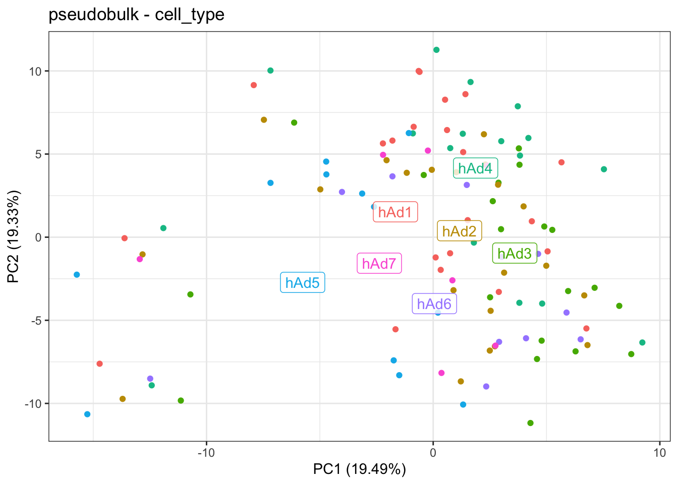
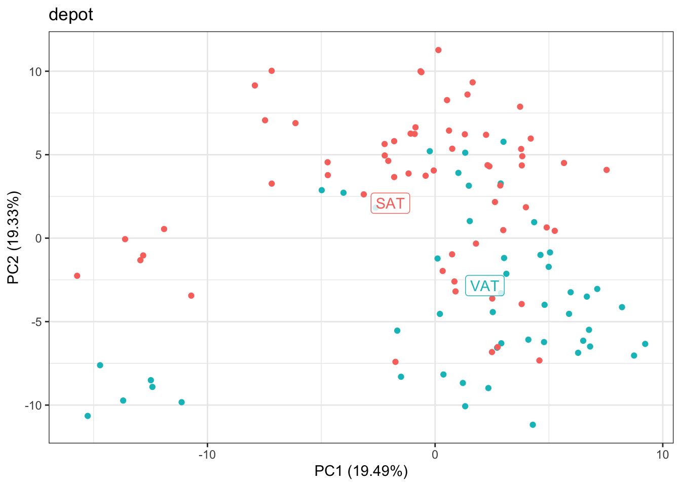
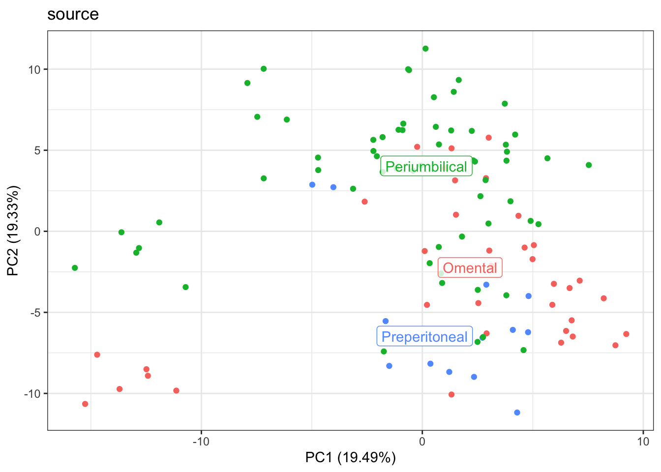
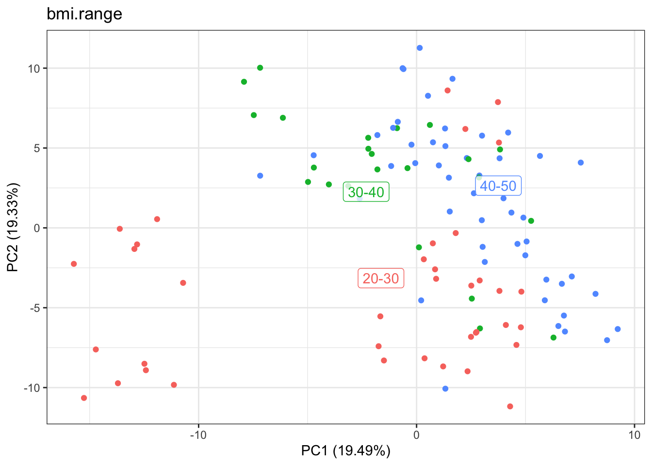
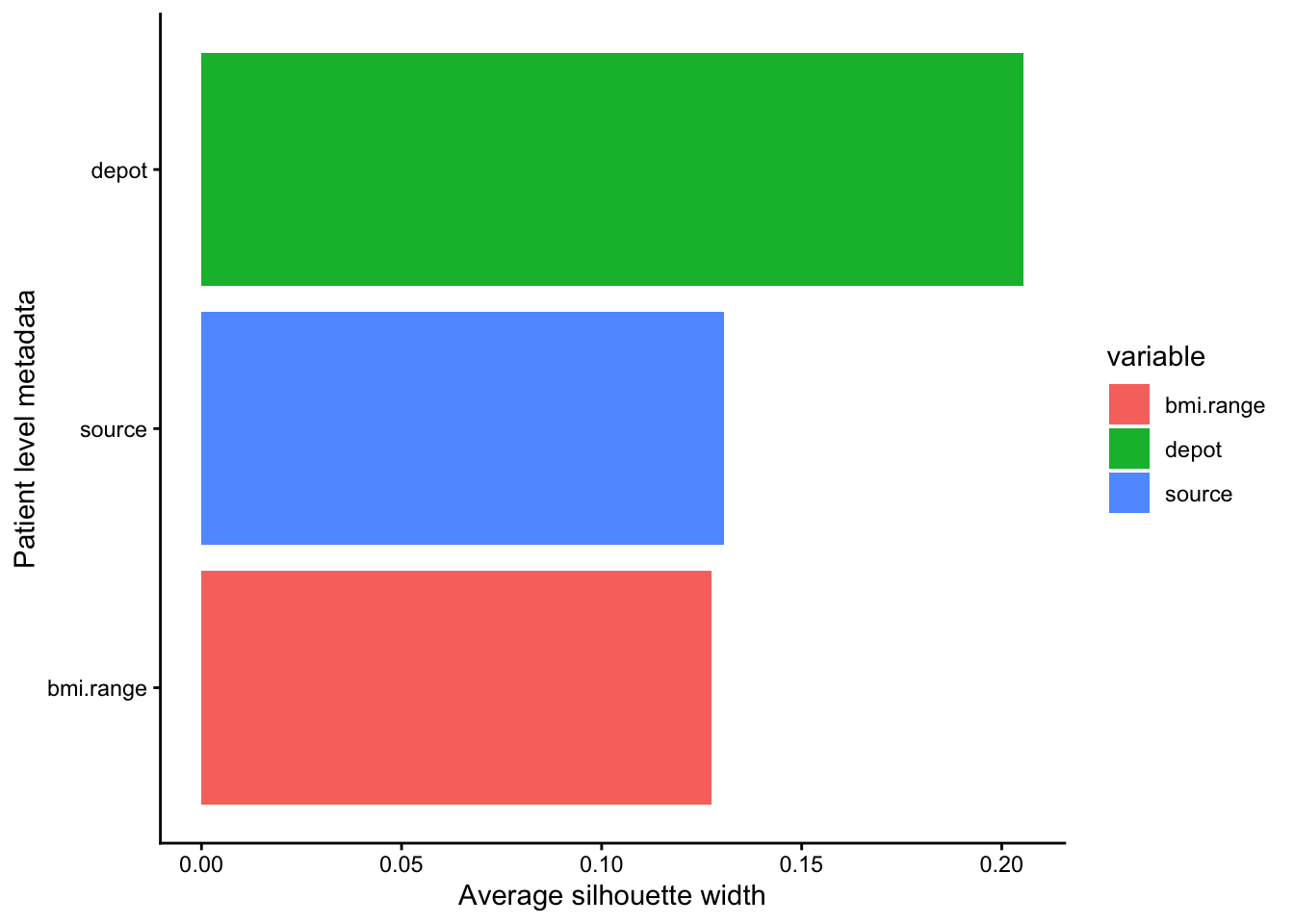
We can see that depot and source separate quite well the samples on the PCA space. We confirm this by measure the silhouette score on the pseudobulk space.

library(purrr)
# get Cosine distance across pseudobulk aggregates
sceval_adipo <- run_dissimilarity(
  sceval_adipo,
  method = "Pseudobulk:Cosine",
  reduction = TRUE,
  verbose = FALSE
)
pseudobulk_cosine_dist <- sceval_adipo@dissimilarity$`Pseudobulk:Cosine`@dissimilarity
# compute silhouette score for the different vars
silhouette_summary <- map_dfr(
  sample_vars,
  function(v) {

    sil <- cluster::silhouette(
      x = as.numeric(as.factor(col_annot[[v]])),
      dist = pseudobulk_cosine_dist
    )

    tibble(
      variable = v,
      mean_silhouette = mean(sil[, "sil_width"], na.rm = TRUE),
      median_silhouette = median(sil[, "sil_width"], na.rm = TRUE)
    )
  }
)

ggplot(
  silhouette_summary,
  aes(
    x = reorder(variable, mean_silhouette),
    y = mean_silhouette,
    fill = variable
  )
) +
  geom_col() +
  coord_flip() +
  theme_classic() +
  labs(y = "Average silhouette width",
       x = "Patient level metadata")

# Visualize MDS of cosine distances
sceval_adipo@dissimilarity$`Pseudobulk:Cosine`@ident$cell_type <- col_annot$depot
plot_mds(sceval_adipo)

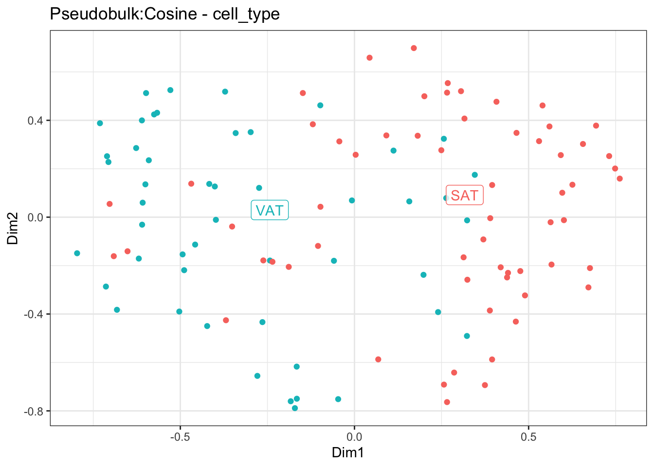
Overall, these findings suggest that: 1) the adipocyte subpopulations proposed by the authors do not represent cell types that are reproducibly recovered across patients; and 2) adipocytes from VAT and SAT show marked gene expression differences.

8.2 Reannotate adipocytes subpopulations

Based on this, we next classify adipocytes into SAT and VAT.

md_depot <- seu_chromv3@meta.data %>%
  mutate(
    fine_annotation_new = case_when(
      cell_type2 == "adipocyte" ~ paste(cell_type2, depot, sep = "."),
      TRUE ~ cell_type
    )
  )
seu_chromv3@meta.data <- md_depot

Let’s explore if categorizing adipocytes based on their depot of origin is reproducible across samples using scTypeEval pipeline. Consider that most individuals contain samples from both SAT and VAT, hence the similarity between them is still present.

sceval_depot <- create_scTypeEval(seu_chromv3)
ident <- "fine_annotation_new" # author's fine annotation

sceval_depot <- run_processing_data(
  scTypeEval = sceval_depot,
  ident = ident, # in this case broad annotation
  sample = "individual",
  min_samples = 5,
  min_cells = 10,
  verbose = FALSE
)

sceval_depot <- run_hvg(
  scTypeEval = sceval_depot,
  ngenes = 2000,
  sample = TRUE,
  aggregation = "single-cell",
  black_list = blacklist_genes,
  ncores = 4,
  verbose = FALSE
)
# remove data from single-cell grouping as we don't need it
sceval_depot@data$`single-cell` <- NULL
sceval_depot <- run_pca(
  scTypeEval = sceval_depot,
  ndim = 30,
  verbose = FALSE
)

8.3 Compute dissimilarities (run_dissimilarity)

sceval_depot <- run_dissimilarity(
  sceval_depot,
  method = "recip_classif:Match",
  reduction = FALSE,
  ncores = 4,
  verbose = FALSE
)

sceval_depot <- run_dissimilarity(
  sceval_depot,
  method = "Pseudobulk:Cosine",
  reduction = TRUE,
  verbose = FALSE
)

# Visualize reciprocal classification match (RCM) plot
plot_heatmap(sceval_depot,
            dissimilarity_slot = "recip_classif:Match", 
            sort_consistency = "silhouette",
            sort_similarity = "Pseudobulk:Cosine") +
  ggtitle("RCM plot - Rennotation")

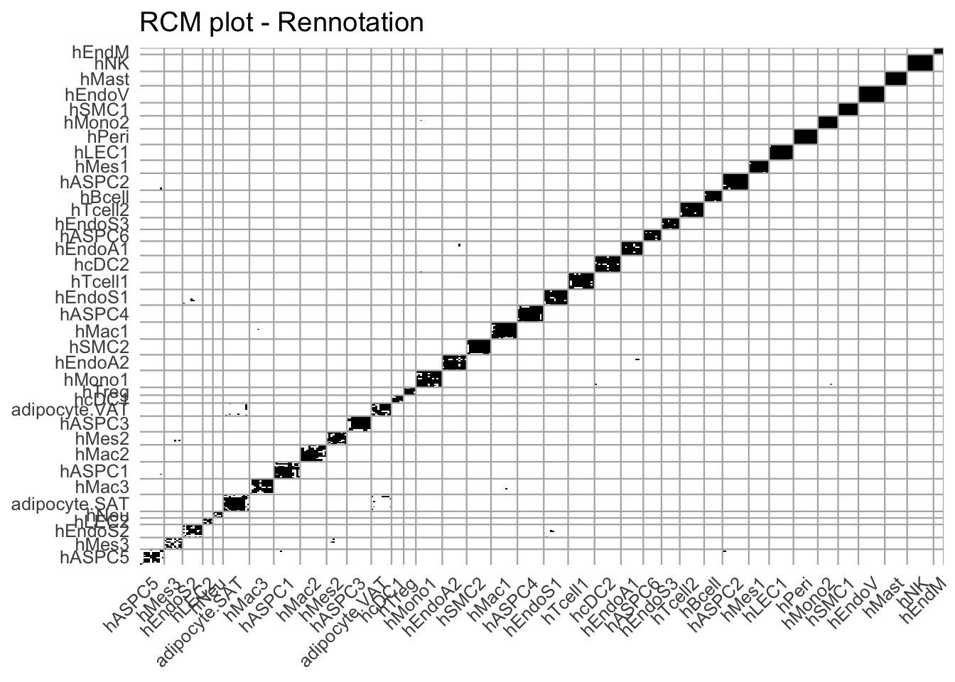
We can see on the RCM plot that the new adipocytes subtypes, split into SAT- and VAT derived (adipocyte.SAT and adipocyte.VAT, respectively) show a much larger degree of reproducibility across individuals.

8.4 Compute consistency (get_consistency)

cons_depot_raw <- get_consistency(
  sceval_depot,
  dissimilarity_slot = c("recip_classif:Match", "Pseudobulk:Cosine"),
  consistency_metric = c("silhouette", "2label_silhouette")
)

### Build local/global ISC table
cons_depot <- cons_depot_raw |>
  mutate(method.type = paste(consistency_metric, dissimilarity_method, sep = " | ")) |>
  filter(method.type %in% c(
    "silhouette | recip_classif:Match",
    "2label_silhouette | Pseudobulk:Cosine"
  )) |>
  mutate(
    metric = factor(
      method.type,
      levels = c(
        "silhouette | recip_classif:Match",
        "2label_silhouette | Pseudobulk:Cosine"
      ),
      labels = c("local", "global")
    )
  ) |>
  select(celltype, metric, measure) |>
  pivot_wider(names_from = metric, values_from = measure) |>
  mutate(integrated_isc = local * global) |>
  arrange(integrated_isc)

# Show scatter of global and local ISC
cons_depot %>%
  ggplot(aes(x = local,
             y = global)) +
  # threshold line of figure 5
  geom_vline(
    xintercept = q_local,
    linetype = "dashed",
    linewidth = 0.5,
    alpha = 0.6
  ) +
  geom_hline(
    yintercept = q_global,
    linetype = "dashed",
    linewidth = 0.5,
    alpha = 0.6
  ) +
  # Points
  geom_point(aes(fill = integrated_isc),
             shape = 21,
             size = 3.2,
             stroke = 0.4,
             color = "black",
             alpha = 0.9,
             show.legend = FALSE) +
  
  # Clean blue gradient (Nature-friendly, perceptually smooth)
  scale_fill_gradient(
    low  = "#F7FBFF",
    high = "#08306B"
  ) +
  
  # Repelled labels (better spacing control)
  ggrepel::geom_text_repel(
    aes(label = celltype),
    size = 3.5,
    max.overlaps = 8,
    box.padding = 0.4,
    point.padding = 0.3,
    segment.size = 0.3,
    segment.color = "grey50",
    min.segment.length = 0,
    seed = 22
  ) +
  
  labs(
    x = "ISCL (silhouette on recip_classif:Match)",
    y = "ISCG (2label_silhouette on Pseudobulk:Cosine)",
    title = "WAT Atlas Reannotated cell types in ISC space"
  ) +
  coord_cartesian(clip = "off") +
  theme_classic(base_size = 12)

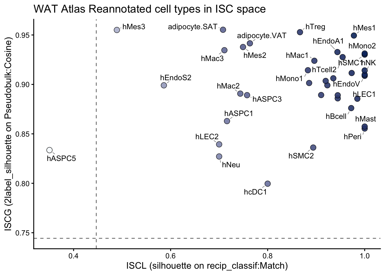
We confirm these findings. New annotations of adipocytes split by the depot of origin increase their ISC.

9 Interpretation

At the broad annotation level, the atlas is highly reproducible across individuals, which suggests that the major adipose, stromal, vascular, and immune compartments are robustly defined in this dataset. In contrast, the fine annotation reveals a clear local inconsistency concentrated in the adipocyte subtypes, consistent with the ISC failure mode described in the paper in which closely related labels cannot be reliably distinguished across samples.

In practice, this means that the original adipocyte fine labels are likely too granular to serve as stable targets for cross-sample comparison or supervised classification. The exploratory analyses further suggest that depot of origin is a stronger and more reproducible source of adipocyte variation than the original subtype labels. Overall, this case study supports using the atlas confidently at the broad level while treating the original adipocyte subtypes with caution and testing simpler, biologically grounded relabeling strategies such as VAT versus SAT.
10 Session information

sessionInfo()
R version 4.6.0 alpha (2026-03-31 r89754)
Platform: aarch64-apple-darwin23
Running under: macOS Tahoe 26.5.1

Matrix products: default
BLAS:   /Library/Frameworks/R.framework/Versions/4.6/Resources/lib/libRblas.0.dylib 
LAPACK: /Library/Frameworks/R.framework/Versions/4.6/Resources/lib/libRlapack.dylib;  LAPACK version 3.12.1

locale:
[1] en_US.UTF-8/en_US.UTF-8/en_US.UTF-8/C/en_US.UTF-8/en_US.UTF-8

time zone: Europe/Zurich
tzcode source: internal

attached base packages:
[1] stats     graphics  grDevices datasets  utils     methods   base     

other attached packages:
[1] purrr_1.2.2        Seurat_5.5.1       SeuratObject_5.4.0 sp_2.2-1          
[5] scTypeEval_1.0.0   ggplot2_4.0.3      tidyr_1.3.2        dplyr_1.2.1       

loaded via a namespace (and not attached):
  [1] RColorBrewer_1.1-3          rstudioapi_0.19.0          
  [3] jsonlite_2.0.0              magrittr_2.0.5             
  [5] spatstat.utils_3.2-3        farver_2.1.2               
  [7] rmarkdown_2.31              vctrs_0.7.3                
  [9] ROCR_1.0-12                 spatstat.explore_3.8-1     
 [11] htmltools_0.5.9             S4Arrays_1.12.0            
 [13] BiocNeighbors_2.6.0         SparseArray_1.12.2         
 [15] sctransform_0.4.3           parallelly_1.48.0          
 [17] KernSmooth_2.23-26          htmlwidgets_1.6.4          
 [19] ica_1.0-3                   plyr_1.8.9                 
 [21] plotly_4.12.0               zoo_1.8-15                 
 [23] igraph_2.3.3                mime_0.13                  
 [25] lifecycle_1.0.5             pkgconfig_2.0.3            
 [27] rsvd_1.0.5                  Matrix_1.7-5               
 [29] R6_2.6.1                    fastmap_1.2.0              
 [31] MatrixGenerics_1.24.0       fitdistrplus_1.2-6         
 [33] future_1.70.0               shiny_1.14.0               
 [35] digest_0.6.39               patchwork_1.3.2            
 [37] S4Vectors_0.50.1            tensor_1.5.1               
 [39] dqrng_0.4.1                 RSpectra_0.16-2            
 [41] irlba_2.3.7                 GenomicRanges_1.64.0       
 [43] beachmat_2.28.0             labeling_0.4.3             
 [45] progressr_1.0.0             spatstat.sparse_3.2-0      
 [47] httr_1.4.8                  polyclip_1.10-7            
 [49] abind_1.4-8                 compiler_4.6.0             
 [51] withr_3.0.3                 S7_0.2.2                   
 [53] BiocParallel_1.46.0         fastDummies_1.7.6          
 [55] MASS_7.3-65                 DelayedArray_0.38.2        
 [57] bluster_1.22.0              tools_4.6.0                
 [59] lmtest_0.9-40               otel_0.2.0                 
 [61] httpuv_1.6.17               future.apply_1.20.2        
 [63] goftest_1.2-3               glue_1.8.1                 
 [65] nlme_3.1-169                promises_1.5.0             
 [67] grid_4.6.0                  Rtsne_0.17                 
 [69] cluster_2.1.8.2             reshape2_1.4.5             
 [71] generics_0.1.4              gtable_0.3.6               
 [73] spatstat.data_3.1-9         data.table_1.18.4          
 [75] metapod_1.20.0              ScaledMatrix_1.20.0        
 [77] BiocSingular_1.28.0         XVector_0.52.0             
 [79] BiocGenerics_0.58.1         spatstat.geom_3.8-1        
 [81] RcppAnnoy_0.0.23            ggrepel_0.9.8              
 [83] RANN_2.6.2                  pillar_1.11.1              
 [85] stringr_1.6.0               limma_3.68.4               
 [87] spam_2.11-4                 RcppHNSW_0.7.0             
 [89] later_1.4.8                 splines_4.6.0              
 [91] lattice_0.22-9              renv_1.2.3                 
 [93] survival_3.8-6              deldir_2.0-4               
 [95] tidyselect_1.2.1            locfit_1.5-9.12            
 [97] SingleCellExperiment_1.34.0 scuttle_1.22.0             
 [99] miniUI_0.1.2                pbapply_1.7-4              
[101] knitr_1.51                  gridExtra_2.3.1            
[103] IRanges_2.46.0              Seqinfo_1.2.0              
[105] edgeR_4.10.1                SummarizedExperiment_1.42.0
[107] scattermore_1.2             stats4_4.6.0               
[109] xfun_0.60                   Biobase_2.72.0             
[111] statmod_1.5.2               matrixStats_1.5.0          
[113] stringi_1.8.7               lazyeval_0.2.3             
[115] yaml_2.3.12                 evaluate_1.0.5             
[117] codetools_0.2-20            tibble_3.3.1               
[119] cli_3.6.6                   uwot_0.2.4                 
[121] xtable_1.8-8                reticulate_1.46.0          
[123] Rcpp_1.1.2                  globals_0.19.1             
[125] spatstat.random_3.5-0       png_0.1-9                  
[127] spatstat.univar_3.2-0       parallel_4.6.0             
[129] dotCall64_1.2               scran_1.40.0               
[131] listenv_1.0.0               viridisLite_0.4.3          
[133] scales_1.4.0                ggridges_0.5.7             
[135] rlang_1.3.0                 cowplot_1.2.0